Show code cell content Hide code cell content

import mmf_setup;mmf_setup.nbinit()
import logging;logging.getLogger('matplotlib').setLevel(logging.CRITICAL)
%matplotlib inline
import numpy as np, matplotlib.pyplot as plt

$\newcommand{\vect}[1]{\mathbf{#1}} \newcommand{\uvect}[1]{\hat{#1}} \newcommand{\abs}[1]{\lvert#1\rvert} \newcommand{\norm}[1]{\lVert#1\rVert} \newcommand{\I}{\mathrm{i}} \newcommand{\ket}[1]{\left|#1\right\rangle} \newcommand{\bra}[1]{\left\langle#1\right|} \newcommand{\braket}[1]{\langle#1\rangle} \newcommand{\Braket}[1]{\left\langle#1\right\rangle} \newcommand{\op}[1]{\mathbf{#1}} \newcommand{\mat}[1]{\mathbf{#1}} \newcommand{\d}{\mathrm{d}} \newcommand{\D}[1]{\mathcal{D}[#1]\;} \newcommand{\pdiff}[3][]{\frac{\partial^{#1} #2}{\partial {#3}^{#1}}} \newcommand{\diff}[3][]{\frac{\d^{#1} #2}{\d {#3}^{#1}}} \newcommand{\ddiff}[3][]{\frac{\delta^{#1} #2}{\delta {#3}^{#1}}} \newcommand{\floor}[1]{\left\lfloor#1\right\rfloor} \newcommand{\ceil}[1]{\left\lceil#1\right\rceil} % The following allows KaTeX to render these for significantly improved % performance on CoCalc. \newcommand{\DeclareMathOperator}[2]{\newcommand{#1}{#2}} \DeclareMathOperator{\Tr}{Tr} \DeclareMathOperator{\erf}{erf} \DeclareMathOperator{\erfi}{erfi} \DeclareMathOperator{\sech}{sech} \DeclareMathOperator{\sn}{sn} \DeclareMathOperator{\cn}{cn} \DeclareMathOperator{\dn}{dn} \DeclareMathOperator{\sgn}{sgn} \DeclareMathOperator{\order}{O} \DeclareMathOperator{\diag}{diag} % \newcommand{\mylabel}[1]{\label{#1}\tag{#1}} \newcommand{\degree}{\circ}$

This cell adds /home/docs/checkouts/readthedocs.org/user_builds/physics-581-the-standard-model/checkouts/latest/src to your path, and contains some definitions for equations and some CSS for styling the notebook. If things look a bit strange, please try the following:

• Choose "Trust Notebook" from the "File" menu.
• Re-execute this cell.
• Reload the notebook.

Dirac Equation

The Essence

Physical objects must transform under specific representations of the Lorentz group. Here we consider four-vectors like \(x^{\mu} = (ct, \vect{x})^T\) and spinors \(\psi_a\), each of which transforms under specific, but different, representations:

\[\begin{gather*} x^{\mu} \rightarrow \Lambda^{\mu}{}_{\nu}x^{\nu}, \qquad x_{\mu} \rightarrow \Lambda_{\mu}{}^{\nu}x_{\nu}, \qquad \psi_a \rightarrow R_{ab}\psi_b, \end{gather*}\]

where \(\mat{\Lambda}(\omega)\) and \(\mat{R}(\omega)\) are matrix representations of the Lorentz group corresponding to the same boosts and rotation parameters \(\omega\).

Though not obvious a-priori, it turns out that the matrix \(\mat{\gamma}^{0}\) needed here is the same as the time-like matrix of \(\mat{\gamma}^{\mu}\) below.

The Dirac equation follows from constructing a Lorentz invariant Lagrangian. Without derivatives, we can form the following term

\[\begin{gather*} \bar{\psi}\psi, \qquad \bar{\psi} = \psi^{\dagger}\mat{\gamma}^0, \qquad \mat{R}^{\dagger}\mat{\gamma}^0\mat{R} = \mat{1}, \end{gather*}\]

where the matrix \(\mat{\gamma}^0\) is needed since the representation \(\mat{R}\) is not unitary.

The Lorentz transform also passively changes the arguments, so four-gradients also transform

\[\begin{gather*} \partial_{\mu}\phi \rightarrow \Lambda_{\mu}{}^{\nu}\partial_{\nu}\phi. \end{gather*}\]

For scalars, we can thus form Lorentz invariant terms with two derivatives, which form the basis for the Klein-Gordon equation

\[\begin{gather*} \mathcal{L} = \frac{1}{2}(\partial_{\mu}\phi\partial^{\mu}\phi - m^2\phi^2), \qquad (\partial_{\mu}\partial^{\mu} + m^2)\phi = 0. \end{gather*}\]

The additional transformation property of spinors \(\psi \rightarrow \mat{R}\psi\) provides another option if we can find matrices \(\mat{\gamma}^{\mu}\) such that

\[\begin{gather*} \mat{\gamma}^{\mu}\mat{R}\Lambda_{\mu}{}^{\nu} = \mat{R}\mat{\gamma}^{\nu}. \end{gather*}\]

This allows us to construct a special derivative that preserves the transformation properties of spinors:

\[\begin{gather*} % https://github.com/mathjax/MathJax/issues/2107#issuecomment-453320217 \def\fslash#1{\mathord{\smash{\mathop{\mat{#1}\strut}\limits^{\smash{\textstyle\lower10pt{\unicode{x2215}}}}}\strut}} \fslash{\partial} = \mat{\gamma}^{\mu}\partial_{\mu},\qquad \fslash{\partial}\psi \rightarrow \mat{R}\,\fslash{\partial}\psi. \end{gather*}\]

This allows us to form a Lorentz invariant Lagrangian with a single derivative that forms the basis for the Dirac equation:

\[\begin{gather*} \mathcal{L} = \bar{\psi}\I\fslash{\partial}\psi - m\bar{\psi}\psi, \qquad (\I\fslash{\partial} - m)\psi = 0. \end{gather*}\]

Rotations

Here \(\varepsilon_{ijk}\) is the Levi-Civita symbol which effects the cross product:

\[\begin{gather*} [\vect{\theta}\times\vect{B}]_i = \varepsilon_{iaj}\theta_aB_j = [\mat{\vect{\theta}\times}]_{ij}B_j. \end{gather*}\]

We start with some group theory for rotations. Active rotations about the axis \(\vect{\theta}\) of magnitude \(\theta = \abs{\theta}\) in 3D can be effected by the following linear transformations, which form a faithful representation of the SO(3) group:

\[\begin{gather*} \mat{R}_{\vect{\theta}} = e^{\mat{\vect{\theta}\times}}, \qquad [\mat{\vect{\theta}\times}]_{ij} = \varepsilon_{iaj}\theta_a. \end{gather*}\]

From this, we can determine the elements of the corresponding Lie Algebra by expanding about the origin to linear order in \(\theta\):

\[\begin{gather*} \mat{R}_{\vect{\theta}} = e^{\mat{\vect{\theta}\times}} = \mat{1} + \mat{\vect{\theta}\times} + O(\theta^2). \end{gather*}\]

I remember these as follows: \(\mat{T}_{k}\) has zeros on both rows and columns \(i=j=k\). The other \(2\times 2\) block is anti-symmetric with \(\mat{T}_{y}\) having the opposite sign as in the formula for a determinant. To get the sign, act on a vector: Under active rotations, \(\mat{T}_{z}\uvect{x} = \uvect{y}\) while \(\mat{T}_{z}\uvect{y} = -\uvect{y}\):

The three generators are \([\mat{T}_{k}]_{ij} = \varepsilon_{ikj}\):

\[\begin{gather*} \mat{T}_{x} = \begin{pmatrix} 0 & 0 & 0\\ 0 & 0 & -1\\ 0 & 1 & 0 \end{pmatrix}, \qquad \mat{T}_{y} = \begin{pmatrix} 0 & 0 & 1\\ 0 & 0 & 0\\ -1 & 0 & 0 \end{pmatrix}, \qquad \mat{T}_{z} = \begin{pmatrix} 0 & -1 & 0\\ 1 & 0 & 0\\ 0 & 0 & 0 \end{pmatrix}. \end{gather*}\]

Rotations are obtained from the algebra by exponentiating:

\[\begin{gather*} \mat{R}_{\vect{\theta}} = e^{\vect{\theta}\cdot\vect{\mat{T}}}. \end{gather*}\]

For rotations in 3D, this notation make sense, but in particle physics a different convention is used that more closely connects with quantum mechanics. The generators \(\mat{T}_a = - \mat{T}_a^T\) are anti-symmetric, but in physics, these will correspond to observables like angular momentum which need to be Hermitian.

Thus, the convention in particle physics is to include a factor of \(\I\):

\[\begin{gather*} \mat{L}_{a} = \I\mat{T}_{a},\qquad \mat{R}_{\vect{\theta}} = e^{\vect{\theta}\cdot\vect{\mat{T}}} = e^{\vect{\theta}\cdot\vect{\mat{L}}/\I}. \end{gather*}\]

The resulting generators are now Hermitian:

\[\begin{gather*} \mat{L}_{x} = \I\begin{pmatrix} 0 & 0 & 0\\ 0 & 0 & -1\\ 0 & 1 & 0 \end{pmatrix}, \qquad \mat{L}_{y} = \I\begin{pmatrix} 0 & 0 & 1\\ 0 & 0 & 0\\ -1 & 0 & 0 \end{pmatrix}, \qquad \mat{L}_{z} = \I\begin{pmatrix} 0 & -1 & 0\\ 1 & 0 & 0\\ 0 & 0 & 0 \end{pmatrix}. \end{gather*}\]

With an additional factor of \(\hbar\) (which we set to one in this course), these form a representation of angular momentum.

The group elements are formed from the algebra by exponentiating, which looks like this:

\[\begin{gather*} \mat{R}_{\vect{θ}} = e^{\vect{θ}\cdot\vect{\mat{T}}} = e^{\vect{θ}\cdot\vect{\mat{L}}/\I} \end{gather*}\]

From now on, we will follow the physics convention. Note that the generators can be obtained by expanding the rotation to linear order:

\[\begin{gather*} \mat{R}_{\vect{\theta}} = \mat{1} + \vect{\theta}\cdot\frac{\mat{L}}{\I} + O(\theta^2). \end{gather*}\]

For example, a rotation about the \(z\) axis has the form:

\[\begin{gather*} \mat{R}_{\theta \uvect{z}} = \begin{pmatrix} \cos\theta & -\sin\theta & 0\\ \sin \theta & \cos \theta & 0\\ 0 & 0 & 1 \end{pmatrix} = \mat{1} + \theta \underbrace{ \begin{pmatrix} 0 & -1 & 0\\ 1 & 0 & 0\\ 0 & 0 & 0 \end{pmatrix} }_{\mat{L}_x/\I} + O(\theta)^2. \end{gather*}\]

Lie Algebras

These matrices form a basis for the Lie algebra, which can be defined in terms of the structure constants:

\[\begin{gather*} [\mat{L}_{a}, \mat{L}_{b}] = \I f_{abc}\mat{L}_{c}. \end{gather*}\]

For \(\mathfrak{so}(3)\), we have \(f_{abc} = \epsilon_{abc}\).

The raising and lowing of indices here has no specific significance, but is common so that summed indices are of mixed height. This will be important later when we use the relativistic metric.

Convention in Mathematics

In terms of the anti-symmetric matrices \(\mat{T}_{a}\), we have

\[\begin{gather*} [\mat{T}_{a}, \mat{T}_{b}] = c_{ab}{}^{c} \mat{T}_{c}. \end{gather*}\]

For rotations in 3D, this notation make sense.

Each has their use. For example, since the structure constants are real, if one has a complex representation \(\mat{T}_{a}\) (not purely real), then one can form another complex representation by conjugating \(\overline{\mat{T}}_{a}\). In the second formulation, this requires an additional sign, \(-\overline{\mat{L}}_{a}\), which inequivalent only if \(\mat{L}_{a}\) is not purely imaginary.

Trivial Representation

We start with the trivial representation, which always exists

\[\begin{gather*} \mat{L}_k = \mat{0}. \end{gather*}\]

This is he only one-dimensional representation, since finite numbers compute. It is thus referred to by the number \(\mathbf{1}\).

Adjoint Representation

Note that the adjoint representation is sometimes written:

\[\begin{gather*} [\mat{L}_{a}]_{bc} = \I f_{acb} \end{gather*}\]

with the indices reversed. This simply means that if \(\mat{L}_{a}\) is a representation, then so is \(-\mat{L}_{a}^{T}\), which follows from taking the transpose of the structure equation:

\[\begin{gather*} [\mat{L}_{a}, \mat{L}_{b}]^T = \I f_{abc} \mat{L}_{c}^T\\ = [\mat{L}_{b}^T, \mat{L}_{a}^T] = -[\mat{L}_{a}^T, \mat{L}_{b}^T]\\ [-\mat{L}_{a}^T, -\mat{L}_{b}^T] = \I f_{abc} (-\mat{L}_{c}^T). \end{gather*}\]

The structure constants also form a matrix representation \(\mat{L}_{a}\) called the adjoint representation (we follow the form in [Georgi, 2019]):

\[\begin{gather*} [\mat{L}_{a}]_{bc} = -\I f_{abc} = -\I \epsilon_{abc}. \end{gather*}\]

It is purely imaginary and has the same dimension as the number of generators. For \(\mathfrak{so}(3)\) this is \(3\) and so this representation is often referred to by the number \(\mathbf{3}\).

Do It!

Show that the adjoint representation defined by the structure factors indeed satisfies the algebra.
Hint: use the Jacobi identity: \(\bigl[\mat{A}, [\mat{B}, \mat{C}]\bigr] + \bigl[\mat{B}, [\mat{C}, \mat{A}]\bigr] + \bigl[\mat{C}, [\mat{A}, \mat{B}]\bigr] = \mat{0}\).

Solution

First we compute:

\[\begin{gather*} \bigl[\mat{L}_{a}, [\mat{L}_{b}, \mat{L}_{c}]\bigr] = \I f_{bcd} [\mat{L}_{a}, \mat{L}_{d}] = - f_{bcd}f_{ade}\mat{L}_{e}. \end{gather*}\]

Summing over permutations of \(\{abc, bca, cab\}\) we can express Jacobi identity as

\[\begin{gather*} f_{bcd}f_{ade} + f_{abd}f_{cde} + f_{cad}f_{bde} = 0. \end{gather*}\]

Now using the adjoint representation \([\mat{L}_{a}]_{bc} = -\I f_{abc}\) and the anti-symmetry \(f_{abc} = -f_{bac}\) implied by the commutator, we can rearrange this as

\[\begin{gather*} \underbrace{ \underbrace{(-\I f_{bcd})}_{[\mat{L}_{b}]_{cd}} \underbrace{(-\I f_{ade})}_{[\mat{L}_{a}]_{de}} - \underbrace{(-\I f_{acd})}_{[\mat{L}_{a}]_{cd}} \underbrace{(-\I f_{bde})}_{[\mat{L}_{b}]_{de}} }_{-[\mat{L}_{b}, \mat{L}_{a}]_{ce}} = -\I f_{abd} \underbrace{(-\I f_{dce})}_{[\mat{L}_{d}]_{ce}},\\ [\mat{L}_{a}, \mat{L}_{b}] = \I f_{abd}\mat{L}_{d}. \end{gather*}\]

This proves that the adjoint representation satisfies the algebra.

Show code cell content Hide code cell content

from scipy.linalg import expm
eps = np.zeros((3, 3, 3)) # Levi-Civita symbol.
eps[0,1,2] = eps[1,2,0] = eps[2,0,1] = 1
eps[2,1,0] = eps[1,0,2] = eps[0,2,1] = -1
Tx, Ty, Tz = T = np.einsum('iaj->aij', eps)
Lx, Ly, Lz = L = 1j*T

def com(A, B):
    return A@B - B@A

assert np.allclose(com(Tx, Ty), Tz)
assert np.allclose(com(Ty, Tz), Tx)
assert np.allclose(com(Tz, Tx), Ty)
assert np.allclose(com(Lx, Ly), 1j*Lz)
assert np.allclose(com(Ly, Lz), 1j*Lx)
assert np.allclose(com(Lz, Lx), 1j*Ly)
print(T.astype(int))

[[[ 0  0  0]
  [ 0  0 -1]
  [ 0  1  0]]

 [[ 0  0  1]
  [ 0  0  0]
  [-1  0  0]]

 [[ 0 -1  0]
  [ 1  0  0]
  [ 0  0  0]]]

Pauli Matrices

The Pauli matrices provide another two-dimensional representation of \(\mathfrak{so}(3)\). To see this, we note:

\[\begin{gather*} \mat{\sigma}_{x} = \begin{pmatrix} 0 & 1\\ 1 & 0 \end{pmatrix}, \qquad \mat{\sigma}_{y} = \begin{pmatrix} 0 & -\I\\ \I & 0 \end{pmatrix}, \qquad \mat{\sigma}_{z} = \begin{pmatrix} 1 & 0\\ 0 & -1 \end{pmatrix} \end{gather*}\]

from which the following properties can be deduced:

\[\begin{gather*} \mat{σ}_{a}\mat{σ}_{b} = \delta_{ab}\mat{1} + \I\varepsilon_{abc}\mat{\sigma}_c,\qquad \Tr\mat{σ}_{a} = 0,\\ [\mat{\sigma}_{a}, \mat{\sigma}_{b}] = 2\I\varepsilon_{abc}\mat{\sigma}_c, \qquad \{\mat{\sigma}_{a}, \mat{\sigma}_{b}\} = 2\delta_{ab}\mat{1}. \end{gather*}\]

Scaling appropriately, we thus see that the following set of matrices form a 2-dimensional representation of \(\mathfrak{s0}(3)\):

\[\begin{gather*} \left[\frac{\mat{\sigma}_{a}}{2}, \frac{\mat{\sigma}_{b}}{2}\right] = \I \varepsilon_{abc}\frac{\mat{\sigma}_c}{2}, \qquad \mat{L}_{a} = \frac{\mat{\sigma}_{a}}{2}. \end{gather*}\]

This is a complex representation referred to by the number \(\textbf{2}\).

As mentioned above, since the structure constants are real, complex representations like this always appear in pairs:

\[\begin{gather*} [-\overline{\mat{L}}_{a}, -\overline{\mat{L}}_{b}] = \I f_{abc}(-\overline{\mat{L}}_{c}). \end{gather*}\]

For \(\mathfrak{so}(3)\), this representation is called \(\mathbf{\bar{2}}\):

\[\begin{gather*} \mat{L}_{a} = \frac{-\overline{\mat{\sigma}}_{a}}{2}. \end{gather*}\]

Show that \(\mathbf{2}\) and \(\mathbf{\bar{2}}\) are equivalent.

I.e. find a matrix \(\mat{S}\) such that

\[\begin{gather*} \mat{S}\mat{\sigma}_{a}\mat{S}^{-1} = -\overline{\mat{\sigma}_{a}}. \end{gather*}\]

Solution

\[\begin{gather*} \mat{S} = \begin{pmatrix} 0 & 1\\ -1 & 0 \end{pmatrix}, \qquad \mat{S}^{-1} = \mat{S}^T = -\mat{S},\qquad [\mat{S}]_{ij} = \varepsilon_{ij}. \end{gather*}\]

This is the 2-dimensional Levi-Civita symbol.

Show code cell source Hide code cell source

σ = np.array([
    [[0, 1],
     [1, 0]],
    [[0, -1j],
     [1j, 0]],
    [[1, 0],
     [0, -1]]])
σbar = -σ.conj() 
assert np.allclose(σ[0]@σ[1], 1j*σ[2])
S = np.array([
    [0, 1],
    [-1, 0]])
Sinv = S.T
assert np.allclose(S @ Sinv, np.eye(2))
assert np.allclose(S @ σ @ S.T, σbar)

Extended Pauli Matrices

Note that, if we include the identity \(\mat{σ}_{0} = \mat{1}\), then Pauli matrices form a basis for Hermitian matrices:

\[\begin{gather*} \mat{A} = \mat{A}^\dagger = a^{\mu}\mat{\sigma}_\mu. \end{gather*}\]

Exponentiating the \(2\) and \(\bar{2}\) representations, we

To Do

This is incomplete.

Gamma Matrices I

Suppose we have some wavefunction \(\psi(\vect{x})\) that transforms under rotations as follows:

\[\begin{gather*} \mathcal{R} \psi(\vect{x}) = \mat{R} \psi(\mat{\Lambda}^{-1}\vect{x}) \end{gather*}\]

where \(\mat{R}\) is some spinor representation (think \(SU(2)\)) and \(\mat{\Lambda}\) is the adjoint representation (\(SO(3)\)) so that derivatives transform as

\[\begin{gather*} \mathcal{R} \nabla_{a}\psi(\vect{x}) = \Lambda_{ab}\nabla_{b}\mat{R}\psi(\mat{\Lambda}^{-1}\vect{x}). \end{gather*}\]

From now on, we will suppress the arguments and just write:

\[\begin{gather*} \psi \rightarrow \mat{R}\psi, \qquad \nabla_{a}\psi \rightarrow \Lambda_{ab}\nabla_{b}\mat{R}\psi. \end{gather*}\]

If \(\mat{R}\) is unitary, then we the following is invariant:

\[\begin{gather*} \psi^\dagger\psi \rightarrow \psi^\dagger\underbrace{\mat{R}^\dagger\mat{R}}_{\mat{1}}\psi = \psi^\dagger\psi. \end{gather*}\]

Can we do something similar with the derivative? One obvious possibility is

\[\begin{align*} (\nabla_{a}\psi)^\dagger (\nabla_{a}\psi) &\rightarrow (\Lambda_{ab}\nabla_{b}\psi)^\dagger \underbrace{\mat{R}^\dagger\mat{R}}_{\mat{1}} (\Lambda_{ac}\nabla_{c}\psi)\\ &= [\underbrace{\mat{\Lambda}^\dagger\mat{\Lambda}}_{\mat{1}}]_{bc}(\nabla_{b}\psi)^\dagger(\nabla_{c}\psi)\\ &= (\nabla_{a}\psi)^\dagger (\nabla_{a}\psi). \end{align*}\]

Another possibility can be formed from a single derivative if we can find a set of matrices \(\mat{\gamma}_{a}\) such that

\[\begin{gather*} \mat{\gamma}_{a}\mat{R}\Lambda_{ab} = \mat{R}\mat{\gamma}_{b} \end{gather*}\]

This allows us to define \(\fslash{\nabla} = \mat{\gamma}_{a}\nabla_{a}\) such that \(\fslash{\nabla}\psi \rightarrow \mat{R}\fslash{\nabla}\psi\) transforms covariantly with \(\mat{R}\):

\[\begin{gather*} \fslash{\nabla}\psi \rightarrow \mat{\gamma}_{a}\Lambda_{ab}\nabla_{b}\mat{R}\psi = \mat{R}\mat{\gamma}_{b}\nabla_{b}\psi = \mat{R}\fslash{\nabla}\psi. \end{gather*}\]

This allows us to form the invariant

\[\begin{gather*} \psi^\dagger \fslash{\nabla}\psi \rightarrow \psi^\dagger \fslash{\nabla}\psi. \end{gather*}\]

To find the matrices \(\mat{\gamma}_{a}\) we expanding the required transformation property to linear order:

\[\begin{gather*} \mat{R} = e^{\vect{\theta}\cdot\vect{\mat{L}}/\I} \approx \mat{1} - \I\theta_{a}\mat{L}_{a}, \qquad \mat{\Lambda} = e^{\vect{\theta}\cdot\vect{\mat{\lambda}}/\I} \approx \mat{1} - \I\theta_{a}\mat{\lambda}_{a},\\ \mat{\gamma}_{a}\mat{R}\Lambda_{ab} = \mat{R}\mat{\gamma}_{b}\\ \mat{\gamma}_{a}(\mat{1} - \I\theta_c \mat{L}_c)(\delta_{ab} - \I \theta_{c}[\mat{\lambda}_c]_{ab}) \approx (\mat{1} - \I\theta_c \mat{L}_c)\mat{\gamma}_{b},\\ -\I\theta_c\Bigl( [\mat{\gamma}_{b},\mat{L}_c] + \mat{\gamma}_{a}[\mat{\lambda}_c]_{ab} \Bigr) = 0,\\ [\mat{\gamma}_{b},\mat{L}_c] + \mat{\gamma}_{a}[\mat{\lambda}_c]_{ab} = 0 \end{gather*}\]

Recall that the generators of the algebra satisfy

\[\begin{gather*} [\mat{L}_{a}, \mat{L}_{b}] = \I f_{abc}\mat{L}_{c}, \qquad [\mat{\lambda}_{a}, \mat{\lambda}_{b}] = \I f_{abc}\mat{\lambda}_{c}. \end{gather*}\]

Hence, if we express the \(\mat{\gamma}_{a}\) matrices in term of the algebra generators, then we have

\[\begin{gather*} \mat{\gamma}_{b} = \mat{L}_{a}c_{ab},\\ [\mat{\gamma}_{b},\mat{L}_c] + \mat{\gamma}_{a}[\mat{\lambda}_c]_{ab} = c_{ab}[\mat{L}_{a},\mat{L}_c] + c_{da}\mat{L}_{d}[\mat{\lambda}_c]_{ab} = 0,\\ c_{ab}\I f_{acd} + \underbrace{c_{da}[\mat{\lambda}_c]_{ab}}_{[\mat{c}\mat{\lambda}_c]_{db}} = 0. \end{gather*}\]

To further elucidate the structure here, recall that the alternative form of the adjoint representation is \([\mat{l}_{c}]_{da} = -\I f_{acd}\). Inserting this gives

\[\begin{gather*} c_{ab}[\mat{l}_{c}]_{da} = [\mat{l}_{c}\mat{c}]_{db} = [\mat{c}\mat{\lambda}_c]_{db}, \qquad \mat{l}_c \mat{c} = \mat{c}\mat{\lambda}_{c}. \end{gather*}\]

In the case of rotations, \(\mat{\lambda}_{c} = \mat{l}_c\) is the adjoint representation, so we can just take \(\mat{c} = \mat{1}\).

However, we know this is not necessary, since, for the Lorentz group, there are 4-dimensional matrices \(\mat{\gamma}^{\mu}\) that do the trick, when the adjoint representation \(\mat{l}_{c}\) is 6-dimensional. The matrix \(\mat{c}\) in this case must be 6×4.

Lorentz Group

In addition to rotations \(\vect{\theta}\), the Lorentz group has boosts. A boost along the \(x\) axis with rapidity \(\eta\) has the form

\[\begin{gather*} \mat{B}_{\eta\hat{x}} = \I \begin{pmatrix} \cosh\eta & \sinh \eta & 0 & 0\\ \sinh \eta & \cosh\eta & 0 & 0\\ 0 & 0 & 1 & 0\\ 0 & 0 & 0 & 1 \end{pmatrix} = e^{\eta\mat{K}_x/\I} \end{gather*}\]

I.e.:

\[\begin{gather*} \mat{J}_{a} = \begin{pmatrix} 1 \\ & \mat{L}_{a} \end{pmatrix}. \end{gather*}\]

The corresponding generators are

\[\begin{gather*} \mat{J}_{x} = \I\begin{pmatrix} 0 & 0 & 0 & 0\\ 0 & 0 & 0 & 0\\ 0 & 0 & 0 & -1\\ 0 & 0 & 1 & 0 \end{pmatrix}, \qquad \mat{J}_{y} = \I\begin{pmatrix} 0 & 0 & 0 & 0\\ 0 & 0 & 0 & 1\\ 0 & 0 & 0 & 0\\ 0 & -1 & 0 & 0 \end{pmatrix}, \qquad \mat{J}_{z} = \I\begin{pmatrix} 0 & 0 & 0 & 0\\ 0 & 0 & -1 & 0\\ 0 & 1 & 0 & 0\\ 0 & 0 & 0 & 0 \end{pmatrix},\\ \mat{K}_{x} = \I \begin{pmatrix} 0 & 1 & 0 & 0\\ 1 & 0 & 0 & 0\\ 0 & 0 & 0 & 0\\ 0 & 0 & 0 & 0 \end{pmatrix}, \qquad \mat{K}_{y} = \I \begin{pmatrix} 0 & 0 & 1 & 0\\ 0 & 0 & 0 & 0\\ 1 & 0 & 0 & 0\\ 0 & 0 & 0 & 0 \end{pmatrix}, \qquad \mat{K}_{z} = \I \begin{pmatrix} 0 & 0 & 0 & 1\\ 0 & 0 & 0 & 0\\ 0 & 0 & 0 & 0\\ 1 & 0 & 0 & 0 \end{pmatrix},\\ \end{gather*}\]

Together, these generate the proper orthochronos Lorentz group:

\[\begin{gather*} \mat{\Lambda}(\vect{\theta}, \vect{\eta}) = e^{(\vect{\theta}\cdot\vect{\mat{J}} + \vect{\eta}\cdot\vect{\mat{K}})/\I},\qquad \vect{\eta} = \uvect{v}\tanh^{-1}\frac{v}{c}, \end{gather*}\]

where the algebra is defined by

\[\begin{gather*} [\mat{J}_{i}, \mat{J}_{j}] = \I \varepsilon_{ijk}\mat{J}_{k}, \qquad [\mat{K}_{i}, \mat{J}_{j}] = \I \varepsilon_{ijk}\mat{K}_{k}, \qquad [\mat{K}_{i}, \mat{K}_{j}] = -\I \varepsilon_{ijk}\mat{J}_{k}. \end{gather*}\]

The defining representation given above defines the 4×4 space-time transformation, but quantum fields can transform under different representations. To classify these, note that these six generators can be rearranged to form a computing \(\mathfrak{su}(2)_L\times\mathfrak{su}(2)_R\) algebra:

\[\begin{gather*} \vect{\mat{J}}^{\pm} = \tfrac{1}{2}(\vect{\mat{J}} \pm \I \vect{\mat{K}}), \qquad [\mat{J}^{\pm}_{i}, \mat{J}^{\pm}_{j}] = \I\varepsilon_{ijk}\mat{J}^{\pm}_{k}, \qquad [\mat{J}^{+}_{i}, \mat{J}^{-}_{j}] = \mat{0}. \end{gather*}\]

Note that the dimension of the \(\mathfrak{su}(2)\) representation with Casimir \(j\) is \(d = 1+2j\). Thus, \(j=0\) is 1 dimensional (scalar), \(j=\tfrac{1}{2}\) is 2-dimensional (spinor), \(j=1\) is 3-dimensional (vector) etc.

Thus, we can label the representations by the pair \((j_+, j_-)\) where \(j_{\pm} = 0, \tfrac{1}{2}, 1, \cdots\) are defined by the Casimirs

\[\begin{gather*} \vect{J}_{\pm}^2 = j_{\pm}(j_{\pm}+1). \end{gather*}\]

The spin-1/2 representations are \(\vect{\mat{J}} = \vect{\mat{\sigma}}/2\) and \(\vect{\mat{K}} = \pm \vect{\mat{\sigma}}/2\I\):

\[\begin{gather*} \newcommand{\spin}{{\small\frac{1}{2}}} \mat{\Lambda}_{(\spin,0)} = e^{(\I\vect{\theta} + \vect{\eta})\cdot\vect{\mat{\sigma}}/2}, \qquad \mat{\Lambda}_{(0, \spin)} = e^{(\I\vect{\theta} - \vect{\eta})\cdot\vect{\mat{\sigma}}/2} = \mat{\Lambda}_{(\spin,0)}^{-1\dagger}, \\ \mat{\Lambda}_{(\spin^{*},0)} = e^{(-\I\vect{\theta} - \vect{\eta})\cdot\vect{\mat{\sigma}^*}/2} = \mat{\Lambda}_{(\spin,0)}^{-1T}, \qquad \mat{\Lambda}_{(0, \spin^*)} = e^{(-\I\vect{\theta} + \vect{\eta})\cdot\vect{\mat{\sigma}}/2} = \mat{\Lambda}_{(\spin,0)}^{*} = \mat{\Lambda}_{({\spin},0)}^{\dagger T}. \end{gather*}\]

Misc.

A scalar wavefunction \(\phi(x^{\mu})\) and its four-gradient transform as

\[\begin{gather*} \phi(x^{\mu}) \rightarrow \phi(\underbrace{\Lambda_{\nu}{}^{\mu}}_{\mathclap{[\mat{\Lambda}^{-1}]^{\mu}{}_{\nu}}}x^{\nu}), \qquad \partial_{\mu}\phi \rightarrow \Lambda_{\mu}{}^{\nu}\partial_{\nu}\phi. \end{gather*}\]

For such a scale, the Lorentz invariant term with four-gradients has two derivatives:

\[\begin{gather*} \partial_{\mu}\phi\partial^{\mu}\phi. \end{gather*}\]

The four-vector transformation satisfies (in matrix then index notation)

\[\begin{gather*} \mat{\Lambda}^T\mat{g}\mat{\Lambda} = \mat{g}, \qquad \Lambda^{\nu}{}_{\mu} g_{\nu\rho}\Lambda^{\rho}{}_{\sigma} = g_{\mu\sigma},\\ \mat{\Lambda}^{-1} = \mat{g}\mat{\Lambda}^T\mat{g}, \qquad [\mat{\Lambda}^{-1}]^{\sigma}{}_{\rho} = g^{\sigma\mu}\Lambda^{\nu}{}_{\mu} g_{\nu\rho} = \Lambda_{\rho}{}^{\sigma}, \qquad \end{gather*}\]

where \(g=\diag(1, -1, -1, -1)\) is the metric. This compactly expressed in Einstein notation where the metric is used to raise and lower indices, and Lorentz invariant quantities can be formed by contracting indices:

\[\begin{gather*} A_{\mu}B^{\mu} = A^{\mu}g_{\mu\nu}B^{\nu} \rightarrow A_{\mu}B^{\mu}. \end{gather*}\]

The wavefunction for an electron has the form \(\psi_a(x^{\mu})\), and transforms as

\[\begin{gather*} \psi(x^{\mu}) \rightarrow \mat{R}\psi(\underbrace{\Lambda_{\nu}{}^{\mu}}_{\mat{\Lambda}^{-1}}x^{\nu}). \end{gather*}\]

The Dirac equation follows from a Lorentz invariant Lagrangian constructed with a single , and the Dirac equation follows

We start

We start from Lorentz transformations which transform four-vectors \(x^{\mu} = (t, \vect{x})^T\) as \(x^{\mu} \rightarrow \Lambda^{\mu}{}_{\nu}x^{\nu}\) where \(\mat{\Lambda}\) is a real 4-dimensional representation of the Lorentz group.

into The electron wavefunction \(\psi_a(\vect{x}, t)\) needs four components

Covariant Formulation

To formulate things covariantly, we define the following four-vectors (now choosing units such that \(c = \hbar = 1\)):

\[\begin{gather*} A^{\mu} = (A^0, \vect{A}), \qquad x^{\mu} = (t, \vect{x}), \qquad p^{\mu} (E, \vect{p}). \end{gather*}\]

Note that the contravariant four-vectors, with a raised index, have the corresponding physical quantities. We now introduce the metric

\[\begin{gather*} g_{\mu\nu} = g^{\mu\nu} = \diag(1, -1, -1, -1). \end{gather*}\]

We follow the conventions in [Langacker, 2017]:

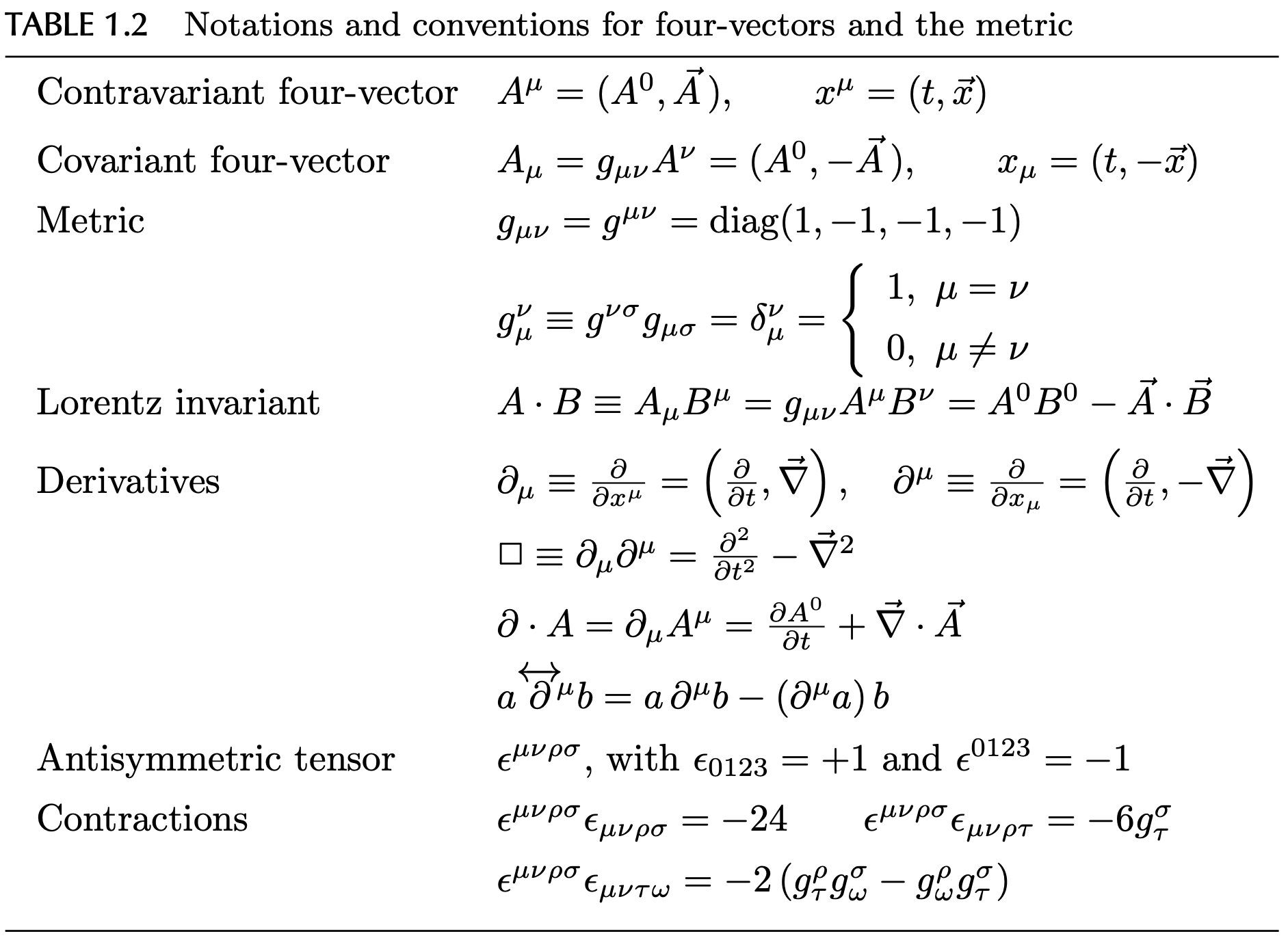
Fig. 2 Table 1.2 from [Langacker, 2017]. Note how the metric \(g_{\mu\nu}\) is used to raise and lower indices, changing the sign of the spatial part in the process.

Using these expressions, we can express the Lorentz transform more covariantly by packaging the angles and rapidities into 4×4 tensor \(\omega_{\rho \sigma}\):

\[\begin{gather*} \theta^{i} = \tfrac{1}{2}\varepsilon^{ijk} \omega_{jk}, \qquad \eta^{i} = \omega^{0i},\\ \omega_{\mu\nu} = \begin{pmatrix} 0 & \vect{\eta}\\ \vect{\eta}^T & \vect{\theta}\cdot\vect{\mat{T}} \end{pmatrix} = \begin{pmatrix} 0 & \eta_x & \eta_y & \eta_z\\ \eta_x & 0 & \theta_z & -\theta_y\\ \eta_y & -\theta_z & 0 & \theta_x\\ \eta_z & \theta_y & -\theta_x & 0\\ \end{pmatrix}. \end{gather*}\]

We similarly package the matrices \(\vect{\mat{J}}\) and \(\vect{\mat{K}}\) into a 4×4 of matrices \(\mat{M}_{\rho\sigma}\):

\[\begin{gather*} \mat{J}^{i} = \tfrac{1}{2}\varepsilon^{ijk}\mat{M}_{jk}, \qquad \mat{K}^{i} = \mat{M}^{0i}, \\ \tfrac{1}{2}\omega^{\rho\sigma}\mat{M}_{\rho\sigma} = \vect{\theta}\cdot\vect{\mat{J}} + \vect{\eta}\cdot\vect{\mat{K}}. \end{gather*}\]

Including the generators of translations \(\mat{P}_{\mu}\) we have the full Poincaré group, which has the algebra

\[\begin{gather*} [\mat{P}_{\mu}, \mat{P}_{\nu}] = 0, \qquad [\mat{M}_{\mu\nu}, \mat{P}_{\rho}] = -\I(g_{\mu\rho}\mat{P}_{\nu} - g_{\nu\sigma}\mat{P}_{\rho}),\\ [\mat{M}_{\mu\nu}, \mat{M}_{\rho\sigma}] = \I(g_{\nu\rho}\mat{M}_{\mu\sigma} - g_{\nu\sigma}\mat{M}_{\mu\rho} - g_{\mu\rho}\mat{M}_{\nu\sigma} + g_{\mu\sigma}\mat{M}_{\nu\rho}). \end{gather*}\]

#:tags: [hide-cell]
J = np.zeros((3, 4, 4), dtype=complex)
J[:, 1:, 1:] = L
K = np.zeros((3, 4, 4), dtype=complex)
for i in [0, 1, 2]:
    K[i, 0, i+1] = K[i, i+1, 0] = 1j
Jx, Jy, Jz = J
Kx, Ky, Kz = K

eta = 0.1
c, s = np.cosh(eta), np.sinh(eta)
assert np.allclose(
    expm(eta*K[0]/1j),
    np.array([
        [c, s, 0, 0],
        [s, c, 0, 0],
        [0, 0, 1, 0],
        [0, 0, 0, 1]]))

def com_(A, B):
    """Return the full set of commutators."""
    return (np.einsum('iab,jbc->ijac', A, B) 
            - np.einsum('ibc,jab->ijac', A, B))

def eps_(A):
    """Return eps_{ijk}A_k."""
    return np.einsum('ijk,kab->ijab', eps, A)
    
assert np.allclose(com_(J, J), 1j*eps_(J))
assert np.allclose(com_(K, J), 1j*eps_(K))
assert np.allclose(com_(K, K), -1j*eps_(J))