Show code cell content Hide code cell content

import mmf_setup;mmf_setup.nbinit()
import logging;logging.getLogger('matplotlib').setLevel(logging.CRITICAL)
%matplotlib inline
import numpy as np, matplotlib.pyplot as plt

$\newcommand{\vect}[1]{\mathbf{#1}} \newcommand{\uvect}[1]{\hat{#1}} \newcommand{\abs}[1]{\lvert#1\rvert} \newcommand{\norm}[1]{\lVert#1\rVert} \newcommand{\I}{\mathrm{i}} \newcommand{\ket}[1]{\left|#1\right\rangle} \newcommand{\bra}[1]{\left\langle#1\right|} \newcommand{\braket}[1]{\langle#1\rangle} \newcommand{\Braket}[1]{\left\langle#1\right\rangle} \newcommand{\op}[1]{\mathbf{#1}} \newcommand{\mat}[1]{\mathbf{#1}} \newcommand{\d}{\mathrm{d}} \newcommand{\D}[1]{\mathcal{D}[#1]\;} \newcommand{\pdiff}[3][]{\frac{\partial^{#1} #2}{\partial {#3}^{#1}}} \newcommand{\diff}[3][]{\frac{\d^{#1} #2}{\d {#3}^{#1}}} \newcommand{\ddiff}[3][]{\frac{\delta^{#1} #2}{\delta {#3}^{#1}}} \newcommand{\floor}[1]{\left\lfloor#1\right\rfloor} \newcommand{\ceil}[1]{\left\lceil#1\right\rceil} % The following allows KaTeX to render these for significantly improved % performance on CoCalc. \newcommand{\DeclareMathOperator}[2]{\newcommand{#1}{#2}} \DeclareMathOperator{\Tr}{Tr} \DeclareMathOperator{\erf}{erf} \DeclareMathOperator{\erfi}{erfi} \DeclareMathOperator{\sech}{sech} \DeclareMathOperator{\sn}{sn} \DeclareMathOperator{\cn}{cn} \DeclareMathOperator{\dn}{dn} \DeclareMathOperator{\sgn}{sgn} \DeclareMathOperator{\order}{O} \DeclareMathOperator{\diag}{diag} % \newcommand{\mylabel}[1]{\label{#1}\tag{#1}} \newcommand{\degree}{\circ}$

This cell adds /home/docs/checkouts/readthedocs.org/user_builds/physics-581-the-standard-model/checkouts/latest/src to your path, and contains some definitions for equations and some CSS for styling the notebook. If things look a bit strange, please try the following:

• Choose "Trust Notebook" from the "File" menu.
• Re-execute this cell.
• Reload the notebook.

Diagonalizing the Radial Schrödinger Equation

Here we continue our previous explorations of numerical methods for solving the radial Schrödinger Equation, trying to overcome some of the shortcomings seen there. We will focus on problems with a Coulomb potential that has both the mild singularity at \(r=0\) and the long tail \(V \sim 1/r\):

\[\begin{gather*} \Biggl( \frac{-\hbar^2}{2m}\biggl(\diff[2]{}{r} + \frac{l(l+1)}{r^2}\biggr) + V(r) - E \Biggr)u(r) = 0. \end{gather*}\]

Note that we can choose units where \(\alpha = \hbar = m = 1\) so that

\[\begin{gather*} 1 = \underbrace{a = \frac{\hbar^2}{m\alpha}}_{\text{length}} = \underbrace{\frac{\alpha}{l}}_{\text{energy}},\\ E_{ln} = \frac{-1}{2n^2}. \end{gather*}\]

There are no dimensionless parameters in this theory. The principal quantum number \(n = n_r + l + 1\) where \(n_r\) is the number of nodes in the wavefunction. The quantum number \(n_r \in \{0, 1, \cdots\}\) is the usual label with \(n_r =0\) being the lowest-energy state with fixed \(l\).

Coulomb Potential

For testing we use the exact energies for the non-relativistic hydrogen atom:

\[\begin{gather*} V(r) = \frac{-\alpha}{r}, \qquad E_{ln} = \frac{-m\alpha^2/\hbar^2}{2n^2} = \frac{-\hbar^2}{2ma^2n^2},\\ u_{ln}(r) = \sqrt{\left(\frac{2}{na}\right)^3\frac{(n-l-1)!}{2n(n+l)!}} re^{-r/na} \left(\frac{2r}{na}\right)^{l} L_{n-l-1}^{(2l+1)}\left(\frac{2r}{na}\right),\\ a = \frac{\hbar^2}{m \alpha},\qquad L_{n}^{(\alpha)}(x) = \frac{x^{-\alpha}}{n!}\left(\diff{}{x} - 1\right)^{n}x^{n+\alpha}. \end{gather*}\]

where \(m\) is the reduced mass \(m = m_em_p/(m_e+m_p)\), \(a\) is the reduced Bohr radius, \(L_{n-l-1}^{(2l+1)}(\rho)\) is a generalized Laguerre polynomial of degree \(n-l-1\), and \(Y_{l}^{m}(\theta, \phi)\) is a spherical harmonic function of degree \(l\) and order \(m\). The full 3D eigenstates are:

\[\begin{gather*} \psi_{n,l,m}(r, \theta, \phi) = u_{nl}(r)Y_{l}^{m}(\theta, \phi). \end{gather*}\]

The states in these formulae are classified by the following quantum numbers:

• \(n \in \{1, 2, 3, \dots\}\): principal quantum number,

• \(l \in \{0, 1, 2, \dots, n-1\}\): azimuthal quantum number. These are sometimes referred to by orbital terminology S (\(l=0\)), P (\(l=1\)), D (\(l=2\)) etc. Here we focus on the S-wave properties \(l=0\) which are spherically symmetric.

• \(m \in \{-l, -l+1, \dots, l-1, l\}\): magnetic quantum number,

Note: Orthogonality between different values of \(l\) is enforced by the spherical harmonics. The radial wavefunctions are orthogonal in the following sense:

\[\begin{gather*} \braket{u_{nl}|u_{ml}} = \int_0^{\infty} u_{nl}^{*}(r)u_{ml}(r)\d{r} = \delta_{mn}. \end{gather*}\]

We now check these properties numerically.

Show code cell source Hide code cell source

from scipy.special import genlaguerre as L, factorial
from scipy.integrate import quad

class Coulomb:
    m = alpha = hbar = 1
    a = hbar**2/m/alpha

    def get_u(self, r, n, l=0):
        a = self.a
        A = np.sqrt((2/n/a)**3*factorial(n-l-1)/2/n/factorial(n+l))
        rho = 2*r/n/a
        return A*r*np.exp(-rho/2)*rho**l*L(n-l-1, 2*l+1)(rho)

    def get_E(self, n, l=0):
        return -self.hbar**2/2/self.m/self.a**2/(1+l+n)**2

coulomb = Coulomb()

# Check orthonormality

N = 10
def f(r):
    return (coulomb.get_u(r, n, l).conj() * coulomb.get_u(r, m, l))

for n in range(1, N+1):
    for m in range(1, n+1):
        for l in range(min(m, n)):
            res = quad(f, 0, np.inf)[0]
            if m == n:
                assert np.allclose(res, 1)
            else:
                assert np.allclose(res, 0)

r = np.linspace(0, 60, 1000)[1:]
fig, ax = plt.subplots()
for l in range(3):
    for n in range(l+1, 5):
        u_r = coulomb.get_u(r, n=n, l=l)
        ax.plot(r, u_r, ls=['-', '--', ':', '-.'][l], c=f"C{n}",
                label=f"{n=}, {l=}")
ax.set(xlabel="$r$", ylabel="$u(r)$") 
ax.legend();

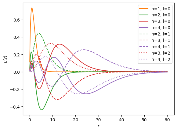
These exact solutions might be used to deal with the singular properties of the Coulomb potential, but we postpone discussing this for now in favour of more general techniques.

Diagonalization

Our diagonalization approach did not work very well before, most likely because of the singularities and long-range tail of the Coulomb potential. One approach for dealing with this is to use the exact solutions above as a basis, and to expand any other terms. This can work quite well, but computing the matrix elements

import scipy.linalg
import scipy as sp

# Hydrogen atom
N = 64*8
R = 20.0
a = R/N
n = np.arange(N)
r = (n + 1)*a

N_states = 30
hbar = m = alpha = 1

Vr = -alpha/r
l = 0
En = -m*alpha**2/hbar**2/2/(1+l+n)**2

D2 = (np.diag(np.ones(N-1), k=1) 
      -2*np.diag(np.ones(N)) 
      + np.diag(np.ones(N-1), k=-1))

I = (np.diag(np.ones(N-1), k=1) 
     + 10*np.diag(np.ones(N)) 
     + np.diag(np.ones(N-1), k=-1))/12

V = np.diag(Vr)

fig, axs = plt.subplots(2, 1)

ax = axs[0]

# Finite Difference
H = -hbar**2/2/m * D2/a**2 + V
E, psi = sp.linalg.eig(H)
inds = np.argsort(E.real)
E, psi = E[inds], psi[:, inds]
ax.semilogy(n[:N_states], abs(E/En-1)[:N_states], label="Finite Difference")
print(En[:4])
print(E[:4].real)

axs[1].plot(r, abs(psi[:,0])**2)
axs[1].plot(r, abs(psi[:,1])**2)

# Numerov
H = -hbar**2/2/m * D2/a**2 + I @ V
E, psi = sp.linalg.eig(H, I)
inds = np.argsort(E.real)
E, psi = E[inds], psi[:, inds]
axs[1].plot(r, abs(psi[:,0])**2)
axs[1].plot(r, abs(psi[:,1])**2)
ax.semilogy(n[:N_states], abs(E/En-1)[:N_states], label="Numerov");
print(E[:4].real)

[-0.5        -0.125      -0.05555556 -0.03125   ]
[-0.49980941 -0.12497557 -0.04998816  0.01634702]

[-0.4995119  -0.1249264  -0.04996446  0.01638553]

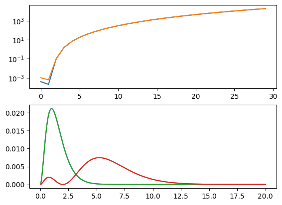
We now see that, although we qualitatively correct solutions, we only have 3 bound states (because our box gets too small), and about 4 places of accuracy, even with a lot of points.

Change of Basis

I think of the basis functions \(\phi_{n}(r)\) as a “unitary matrix” \([\mat{\phi}]_{rn}\) whose first index \(r\) is continuous and whose second index \(n\) is discrete. This is unitary in the sense of

\[\begin{gather*} \mat{\phi}^\dagger \mat{\phi} = \sum_{r}[\mat{\phi}^\dagger]_{mr}[\mat{\phi}]_{rn}\\ = \int \d{r}\;w(r) \phi^*_{m}(r)\phi_{n}(r) = \delta_{mn}. \end{gather*}\]

I.e.

\[\begin{gather*} \sum_{r} \equiv \int \d{r}\; w(r). \end{gather*}\]

If the basis is complete, then we also have

\[\begin{gather*} \mat{\phi}\mat{\phi}^\dagger = \sum_{n}\phi_{n}(r)\phi^*_{n}(r') = \delta(r-r'). \end{gather*}\]

If the basis is finite, however, then this might only be true on some set of discrete abscissa \(r_n\). Now we write:

\[\begin{gather*} \op{H}u(r) = u(r)E, \\ u(r) = \sum_{n}s_n\phi_{n}(r) = \mat{\phi}\ket{s},\\ \underbrace{\mat{\phi}^\dagger \op{H}\mat{\phi}}_{\mat{H}}\ket{s} = \mat{\phi}^\dagger\mat{\phi}\ket{s}E = \ket{s}E,\\ \mat{H}\mat{S} = \mat{S}\mat{E}. \end{gather*}\]

A general strategy is to express the problem in an orthonormal basis \(\ket{\phi_n}\) of functions \(\phi_n(r) = \braket{r|\phi_n}\),

\[\begin{gather*} \braket{\phi_m|\phi_n} = \int\d{r}\; w(r) \phi_m^*(r)\phi_n(r) = \delta_{mn}, \end{gather*}\]

using an inner product with a weight function \(w(r)\). E.g., in spherical coordinates we might take \(w(r) \propto r^2\). One now simply computes the matrix elements of the Hamiltonian and diagonalize:

\[\begin{gather*} \braket{\phi_m|\op{H}|\phi_n} = [\mat{H}]_{mn} = \int\d{r}\; w(r) \phi^*_m(r) \Biggl( \frac{-\hbar^2}{2m}\Bigl(\phi''_n(r) + \frac{l(l+1)}{r^2}\phi_n(r)\Bigr) + V(r)\phi_n(r) \Biggr),\\ \mat{H} = \mat{S}\mat{E}\mat{S}^{-1},\qquad u_n(r) = \sum_{m}\phi_m(r)\mat{S}_{mn}, \end{gather*}\]

where \(\mat{E} = \diag(E_0, E_1, \dots)\). Depending on the complexity of the basis functions, the terms in this integral may be easier or harder to compute.

An obvious application is to use the exact solutions to the Coulomb potential:

\[\begin{gather*} \op{H} = \op{H}_{C} + V_{s}(\op{r}). \end{gather*}\]

Here we demonstrate this technique by computing the lowest 3 eigenvalues for

\[\begin{gather*} V(r) = \underbrace{\frac{-\alpha}{r}}_{V_C} + \underbrace{\frac{\alpha}{a}e^{-r^2/2a^2}}_{V_s}. \end{gather*}\]

coulomb = Coulomb()

l = 0

def get_V(r):
    alpha, a = coulomb.a, coulomb.alpha
    return alpha/a * np.exp(-(r/a)**2/2)

N = 40
V = np.zeros((N, N))
ns = np.arange(1, N+1)

# These loops are quite slow...
for n in ns:
    for m in range(n, N+1):
        def f(r):
            un = coulomb.get_u(r, n, l=l)
            um = coulomb.get_u(r, m, l=l)
            return um.conj()*get_V(r)*un
        V[n-1, m-1] = V[m-1, n-1] = quad(f, 0, np.inf)[0]

H0 = np.diag(coulomb.get_E(n=ns, l=l))
H = H0 + V
E_ = np.linalg.eigvalsh(H)

Es = []
N0 = 3
Ns = 2**np.arange(1+int(np.log2(N0)), 1+int(np.log2(N)))
Es = np.array([np.linalg.eigvalsh(H[:N, :N])[:N0] for N in Ns])
fig, ax = plt.subplots()
ax.loglog(Ns, abs(Es - E_[:N0]), '-+')
ax.set(xlabel="$N$", ylabel="$E$ error", xticks=Ns);

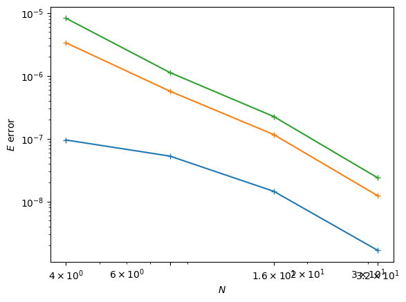
We see that this basis does a reasonable job, but the integrals are quite expensive to compute. For a one-off computation, this should work to generate some data for analysis. (Note: we have only crudely estimated the “correct” answers here by computing in a larger basis, so take the observed scaling with a grain of salt.)

To Do:

• Demonstrate how to use Numba or similar to speed the computation of the overlap integrals so this method becomes feasible.

• Maybe formally study convergence.

DVR Basis

Another approach for diagonalization is to use a discrete variable representation (DVR) basis (sometimes called pseudo-spectral methods). These can be constructed for any orthogonal polynomials (see [Baye and Heenen, 1986]), but we start with the basic formalism, which can also be applied to other orthonormal basis sets, like the Fourier basis.

Slightly more generally, we can define the inner-product in terms of a Lebesque-Stieltjes integral with a measure \(\alpha(x)\), which is any non-decreasing function on the real numbers \(\alpha: \mathbb{R} \mapsto \mathbb{R}\):

\[\begin{gather*} \braket{P_m|P_n} = \int P_m^*(x)P_n(x) \d{\alpha(x)}. \end{gather*}\]

The relationship to the weight function \(w(x)\) is \(\d{\alpha(x)} = w(x)\d{x}\): i.e. \(w(x) = \alpha'(x)\). For example, the Lebesque-Stieltjes with \(\alpha(x) = \Theta(x)\) rigorously defines what we mean by a Dirac delta function weight \(w(x) = \delta(x)\).

To construct a DVR basis, one needs two ingredients:

1. A set of \(N\) orthonormal basis functions \(P_n(x)\).

2. An \(N\)-point Gaussian quadrature rule exact for all linear and quadratic products of the basis functions.

Orthonormality is defined with respect to an inner product

\[\begin{gather*} \braket{P_m|P_n} = \int\d{x}\; w(x)P_m^*(x)P_n(x) = \delta_{mn}, \end{gather*}\]

and the \(N\)-point quadrature rule consists of \(N\) points \(x_i\) and weights \(w_i\) such that

\[\begin{gather*} \int \d{x}\; w(x)f(x) = \sum w_i f(x_i). \end{gather*}\]

For a DVR basis, we need this quadrature formula to be exact for:

1. The functions: \(P_n(x)\).

2. Products: \(P_m^*(x)P_n(x)\).

3. Products with an additional factor of \(x\): \(xP_m^*(x)P_n(x)\). (This is not strictly needed, but ensures that keeping the potential diagonal works reasonably well.)

This will be the case for the orthogonal polynomials, which is why we use the notation \(P_n(x)\), but also holds for the Fourier basis and some other sets with appropriately chosen quadrature rules.

To compare with the literature, note that [Schneider and Nygaard, 2004] uses the notation \(u_n(x) = \sqrt{w(x)}F_n(x)\) so that expectation values are simple

\[\begin{gather*} \braket{u_m|A(x)|u_n} = \int \d{x}\; u_m^*(x) A(x) u_n(x). \end{gather*}\]

This is convenient for numerical work.

In the notation of [Littlejohn et al., 2002], \(K_m = 1/w_m\). They use the following three functions, which differ only by normalization:

\[\begin{gather*} \Delta_n(x) = \sqrt{K_n}F_n(x) = K_n L_n(x),\\ \frac{\braket{\Delta_m|\Delta_n}}{K_m} = \braket{F_m|F_n} = K_m\braket{L_m|L_n} = \delta_{mn}\\ \frac{\Delta_{m}(x_n)}{K_{m}} = \frac{F_{m}(x_n)}{\sqrt{K_m}} = L_{m}(x_n) = \delta_{mn}. \end{gather*}\]

From these ingredients, we construct a set of coordinate basis functions \(F_n(x)\) that are local in the sense that \(F_n(x_m)\) vanishes unless \(m=n\), and that are orthonormal with respect to the coordinate \(x\):

\[\begin{gather*} F_m(x) = \sum_{n} c_{mn}P_n(x), \qquad F_m(x_n) = f_m\delta_{mn}, \\ \braket{F_m|F_n} = \delta_{mn}, \qquad \braket{F_m|x|F_n} = x_m\delta_{mn}. \end{gather*}\]

Using the orthonormality and evaluating the integrals with the quadrature rule, these properties give the relationship:

\[\begin{gather*} c_{mn} = \int \d{x}\; w(x) P_{n}^*(x)F_{m}(x) = \sum_{i} w_i P_{n}^*(x_i)F_{m}(x_i) = w_m P_{n}^*(x_m)f_m,\\ \delta_{mn} = \int \d{x}\; w(x) F_m^*(x)F_n(x) = \sum_{i} w_i F_m^*(x_i)F_n(x_i) = w_m \abs{f_m}^2. \end{gather*}\]

These can be solved, taking \(f_m\) to be real:

\[\begin{gather*} f_m = \frac{1}{\sqrt{w_m}}, \qquad c_{mn} = \sqrt{w_m}P_{n}^*(x_m), \qquad F_{m}(x) = \sqrt{w_m}\sum_{n}P_{n}^*(x_m)P_n(x). \end{gather*}\]

If the last quadrature condition is satisfied, then we have \(\braket{F_m|x|F_n} = x_m\delta_{mn}\), which gets to the essence of these basis, that the potential can be expressed as a diagonal matrix:

\[\begin{gather*} [\mat{V}]_{mn} = \braket{F_m|V(x)|F_n} = V(x_m)\delta_{mn}. \end{gather*}\]

To compute the kinetic energy, we must include factors of \(\sqrt{w(x)}\) in the basis functions:

\[\begin{gather*} u_n(x) = \sqrt{w(x)}F_{n}(x). \end{gather*}\]

Then, the kinetic energy can be evaluated using integration by parts and the quadrature rule. See below for details.

Orthogonal Polynomials

The integral \(\int \d{\alpha(x)}\) is a Lebesque-Stieltjes integral with measure \(\alpha(x)\), which should be a non-decreasing function on the reals. More commonly, we write \(\d{\alpha(x)} = w(x)\d{x}\) where \(w(x) = \alpha'(x)\) is called the weight function, but this is less general/more ambiguous. E.g. \(\alpha(x) = \Theta(x)\) rigorously defines what we mean by a Dirac delta function \(w(x) = \delta(x)\).

One way of constructing a DVR basis is from a set of \(N\) polynomials \(P_n(x)\) (i.e. of maximum degree \(N-1\)) that are orthonormal with respect to a measure \(\alpha(x)\):

\[\begin{gather*} \braket{P_m|P_n} = \int P_m(x)P_n(x) \d{\alpha(x)}. \end{gather*}\]

An \(N\)-point Gaussian quadrature rule is a set of \(N\) points \(x_i\) and weights \(w_i\) such that

\[\begin{gather*} \int P(x)\d{\alpha} = \sum w_i f(x_i) \end{gather*}\]

is exact for all polynomials of degree \(2N-1\) or less. To be used in constructing the DVR basis, the quadrature rule must be exact for polynomials of order \(2(N-1) + 1 = 2N-1\), thus, the Gaussian quadrature provides an acceptable set of \(N\) abscissa and weights for constructing the DVR basis using the formulae above.

To calculate these weights and abscissa, see e.g. §4.6 of Numerical Recipes.

To obtain this order of accuracy, we must be free to choose both the weights and the points. If we want \(x_0\) and/or \(x_{N-1}\) are the endpoints of the integration interval, then we must sacrifice one or two orders:

• Gauss-Radau rules or Radau quadrature fixes one endpoint and is exact up to order \(2N-2\).

• Gauss-Lobatto rules or Lobatto quadrature fixes both endpoints and is exact up to order \(2N-3\).

On the surface, this sees to be a problem for constructing the DVR basis, but as pointed out in [Schneider and Nygaard, 2004], the Radau quadrature based on the Laguerre polynomials is find for solving the radial equation if we exclude the first abscissa \(x_0 = 0\) where \(u(0) = 0\). Thus, we can use an \(N+1\)-point Radau quadrature, exact for polynomials of order \(2N\), and take the \(N\) positive abscissa and weights to construct the DVR basis.

Laguerre-Radau Quadrature

Note that most implementations of \(L_{n}^{(\alpha)}\) are not normalized:

\[\begin{gather*} \int_{0}^{\infty}\d{x}\; x^{\alpha}e^{-x}[L_{n}^{(\alpha)}(x)]^2 \\= \frac{\Gamma(n + \alpha + 1)}{\Gamma(n+1)}. \end{gather*}\]

The generalized Laguerre polynomials \(L_{N}^{(\alpha)}\) are orthogonal on \([0, \infty)\) with weight \(w(x) = x^{\alpha}e^{-x}\). The Radau quadrature abscissa \(x_i\) include \(x_0=0\) and the roots of \(L_{N}^{(\alpha+1)}(x)\), with quadrature weights \(w_i\) [Gautschi, 2000]:

\[\begin{gather*} L_{N}^{(\alpha+1)}(x_i) = 0, \qquad w_{0} = \frac{\Gamma(\alpha+1)}{{N+\alpha+1} \choose {N}}, \qquad w_{i} = \frac{\Gamma(\alpha+1)}{N+\alpha+1} {N+\alpha \choose N} \frac{1}{[L_{N}^{(\alpha)}(x_i)]^2}. \end{gather*}\]

Show code cell source Hide code cell source

from warnings import warn

from itertools import product

import numpy as np
from scipy.integrate import quad

from phys_581.dvr import roots_genlaguerre_radau, LaguerreRadauDVR

dvr = LaguerreRadauDVR(N=10)
ns = range(dvr.N+1)
for m in ns:
    def f(r):
        return dvr.get_w(r)*dvr.F(r,m)
    assert np.allclose(quad(f, 0, np.inf)[0], sum(dvr.w*dvr.F(dvr.r, m)))

for m, n in product(ns, ns):
    # Orthonormality of P
    def f(r):
        return dvr.get_w(r)*dvr.P(r,m)*dvr.P(r,n)
    np.allclose(quad(f, 0, np.inf)[0], 1 if n == m else 0)

for m, n in product(ns, ns):
    def f(r):
        return dvr.get_w(r)*dvr.F(r,m)*dvr.F(r,n)
    assert np.allclose(quad(f, 0, np.inf)[0], sum(dvr.w*dvr.F(dvr.r, m)*dvr.F(dvr.r, n)))

for m, n in product(ns, ns):
    def f(r):
        return dvr.get_w(r)*dvr.F(r,m)*dvr.F(r,n,d=1)
    assert np.allclose(quad(f, 0, np.inf)[0], sum(dvr.w*dvr.F(dvr.r, m)*dvr.F(dvr.r,n,d=1)))

for m, n in product(ns, ns):
    def f(r):
        return dvr.get_w(r)*dvr.F(r,m,d=1)*dvr.F(r,n,d=1)
    assert np.allclose(quad(f, 0, np.inf)[0], sum(dvr.w*dvr.F(dvr.r, m,d=1)*dvr.F(dvr.r,n,d=1)))

#for m in range(1, dvr.N+1):
#    def f(r):
#        return dvr.get_w(r)*dvr.F(r, m)*r
#    assert np.allclose(quad(f, 0, np.inf)[0], sum(dvr.w*dvr.F(dvr.r, m)*dvr.r))

for m, n in product(ns, ns):
    def f(r):
        return (dvr.get_w(r)
                * ((dvr.alpha - r)/2/r * dvr.F(r,m,d=0) + dvr.F(r,m,d=1))
                * ((dvr.alpha - r)/2/r * dvr.F(r,n,d=0) + dvr.F(r,n,d=1)))
    assert np.allclose(quad(f, 0, np.inf)[0]/2, dvr.T[m,n])

Kinetic Energy

To compute the kinetic energy we note that the basis functions are a sum of terms of the form

\[\begin{gather*} f(r) = \overbrace{\sqrt{r^{\alpha}e^{-r}}}^{\sqrt{w}}L(r),\qquad f'(r) = \sqrt{w(r)}\left(\frac{\alpha - r}{2r}L + L'(r)\right). \end{gather*}\]

Thus, we can compute the kinetic energy matrix using the quadrature forumlae:

\[\begin{gather*} K_{mn} = \braket{u_m|\left(-\tfrac{1}{2}\diff[2]{}{r}\right)|u_n} = \frac{1}{2}\int\d{r}\; u_{m}'(r) u_{n}'(r)\d{r} = \frac{1}{2}\sum_{i} w_i \frac{u_{m}'(r_i) u_{n}'(r_i)}{w(r_i)} \end{gather*}\]

Detailed expressions for \(N=1\) (used to check code).

Getting everything working here is quite challenging as there are lots of places for making mistakes. Ultimately we should have a comprehensive set of tests, but initially it is helpful to work with a small basis. Working through these and explicitly checking the code helped me find several subtle issues. We take \(N=1\) with two abscissa.

With \(\alpha = 0\), we have explicitly:

\[\begin{align*} P_0(r) = L_0^{(\alpha)}(r) &= 1\\ P_1(r) = L_1^{(\alpha)}(r) &= 1 +\alpha - r = 1-r\\ L_{1}^{(\alpha+1)}(r) &= 2+\alpha-r = 2 - r\\ w_0 = w_1 &= \frac{1}{2},\\ \mat{C} &= \frac{1}{\sqrt{2}}\begin{pmatrix} 1 & 1\\ 1 & -1 \end{pmatrix},\\ F_0(r) &= \frac{P_0(r) + P_1(r)}{\sqrt{2}} = \frac{2-r}{\sqrt{2}}\\ F_1(r) &= \frac{P_0(r) - P_1(r)}{\sqrt{2}} = \frac{-r}{\sqrt{2}}\\ u_1(r) &= \tfrac{-1}{\sqrt{2}}re^{-r/2}. \end{align*}\]

The abscissa are \(r_0 = 0\) and \(r_1 = 2\), the latter being the roots of \(L_{N}^{(\alpha+1)}(r)\).

For \(\alpha=1\) we have

\[\begin{align*} P_0(r) = L_0^{(1)}(r) &= 1\\ P_1(r) = \tfrac{1}{\sqrt{2}}L_1^{(1)}(r) &= \frac{2 - r}{\sqrt{2}}\\ L_{1}^{(2)}(r) &= 3 - r\\ (w_0, w_1) &= (\tfrac{1}{3}, \tfrac{2}{3}),\\ \mat{C} &= \frac{1}{\sqrt{3}} \begin{pmatrix} 1 & \sqrt{2}\\ \sqrt{2} & -1 \end{pmatrix},\\ F_0(r) = \frac{P_0(r) + \sqrt{2}P_1(r)}{\sqrt{3}} &= \frac{3 - r}{\sqrt{3}},\\ F_1(r) = \frac{\sqrt{2}P_0(r) - P_1(r)}{\sqrt{3}} &= \frac{r}{\sqrt{6}},\\ u_0(r) &= \tfrac{1}{\sqrt{3}}(3-r)\sqrt{r}e^{-r/2},\\ u_1(r) &= \tfrac{1}{\sqrt{6}}r\sqrt{r}e^{-r/2} \end{align*}\]

Thus, despite the fact that the \(\alpha = 1\) basis has \(L_{n}^{(1)}\) basis polynomials, the factor of \(\sqrt{r}\) ruins the convergence.

Note that for \(m = \alpha = \hbar = 1\), the first few state for Hydrogen are

\[\begin{gather*} u_{01}(r) = 2re^{-r}L_{0}^{(1)}(2r) = 2re^{-r}, \\ u_{02}(r) = \tfrac{1}{2\sqrt{2}} re^{-r/2}L_{1}^{(1)}(r) = \tfrac{1}{4}e^{-r/2}(2-r)r. \end{gather*}\]

One might be able to look at the quantitative convergence using this idea. For example, to have accuracy to order \(\epsilon^3\), three of the highest basis function in the expansion would now be outside of the basis since they have an extra factor of \(r^3\). There may be a path towards good error estimates here, but we resort to some experiments.

One final comment: We have expressed our basis in some sort of “natural” units where \(r\) is dimensionless. This is no good for physics. Instead, we must choose a length scale \(a\) in which to express our problem. Once we choose, this scale, the basis can be used by scaling \(r\rightarrow r/a\) to be dimensionless, and then adding the missing factors \(\mat{K}/a^2\) to the kinetic energy. To choose \(a\), note that the quadrature is exact for radial wavefunctions of the form (setting \(\alpha = 0\) here)

\[\begin{gather*} u(r) \propto e^{-r/2a}L\left(\frac{r}{a}\right). \end{gather*}\]

This might indicate that an optimal choice is \(a \propto n \propto 1/\sqrt{-E}\) for Coulomb-like potentials. We will explore how well this works below, but note that choosing a slightly incorrect \(a\) still works well because

\[\begin{gather*} e^{-r/2a + \epsilon r} = e^{-r/2a}\left(1 + \epsilon r + \frac{\epsilon^2}{2!}r^2 + \cdots\right). \end{gather*}\]

Thus, the errors induce polynomial factors that are well represented in the basis.

Example: Coulomb-like Potentials.

Here we use the Laguerre-Radau approach described above to solve for states in a Coulomb-like potential.

Show code cell source Hide code cell source

def get_Es(N=32, a=1.0):
    dvr = LaguerreRadauDVR(N=N, alpha=0)
    H = dvr.T[1:, 1:] + np.diag(-a/dvr.r[1:])
    En = np.linalg.eigvalsh(H)/a**2
    return En


Nstates = 15
a = 1.0
Nmax = 200
ns = 1+np.arange(Nstates)
E_exact = -1/2/ns**2

Ns = np.arange(Nstates, Nmax+1, 4)
errs = [get_Es(N, a=a)[:Nstates]/E_exact - 1 for N in Ns]

fig, ax = plt.subplots()
ax.semilogy(Ns, np.abs(errs), '-+')
ax.legend(1+np.arange(Nstates))
ax.set(xlabel="Basis size $N$", ylabel="Relative error",
       title=f"Lowest {Nstates} states: ${a=}$");

/home/docs/checkouts/readthedocs.org/user_builds/physics-581-the-standard-model/checkouts/latest/src/phys_581/dvr.py:40: RuntimeWarning: overflow encountered in square
  gamma(alpha + 1) / (n + alpha + 1) * comb(n + alpha, n) / Lx**2,
/home/docs/checkouts/readthedocs.org/user_builds/physics-581-the-standard-model/checkouts/latest/src/phys_581/dvr.py:149: UserWarning: 1 zero weights (out of N=187)
  warn(f"{sum(w==0)} zero weights (out of {N=})")
/home/docs/checkouts/readthedocs.org/user_builds/physics-581-the-standard-model/checkouts/latest/src/phys_581/dvr.py:149: UserWarning: 1 zero weights (out of N=191)
  warn(f"{sum(w==0)} zero weights (out of {N=})")

/home/docs/checkouts/readthedocs.org/user_builds/physics-581-the-standard-model/checkouts/latest/src/phys_581/dvr.py:149: UserWarning: 2 zero weights (out of N=195)
  warn(f"{sum(w==0)} zero weights (out of {N=})")
/home/docs/checkouts/readthedocs.org/user_builds/physics-581-the-standard-model/checkouts/latest/src/phys_581/dvr.py:149: UserWarning: 3 zero weights (out of N=199)
  warn(f"{sum(w==0)} zero weights (out of {N=})")

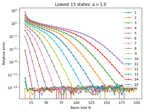
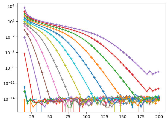
Here we see the convergence of the lowest 15 states as a function of basis size \(N\). Around \(N \approx 180\), numerical errors in the computation start to corrupt the basis, leading to zero weights (see warnings), overflows, etc. While there might be ways to mitigate this (we have included one in the code, using exact integer math for some of the coefficients), it is probably not worth pursuing this direction.

Instead, it us much more profitable to explore adjusting the length scale \(a\).

Show code cell source Hide code cell source

Nstates = 15
a = 1.0
Nmax = 200
ns = 1+np.arange(Nstates)
E_exact = -1/2/ns**2

Ns = np.arange(Nstates, Nmax+1, 4)
errs = [get_Es(N, a=a)[:Nstates]/E_exact - 1 for N in Ns]

fig, ax = plt.subplots()
ax.semilogy(Ns, np.abs(errs), '-+')
ax.legend(1+np.arange(Nstates), loc='left')
ax.set(xlabel="Basis size $N$", ylabel="Relative error",
       title=f"Lowest {Nstates} states: ${a=}$");

---------------------------------------------------------------------------
ValueError                                Traceback (most recent call last)
Cell In[7], line 12
     10 fig, ax = plt.subplots()
     11 ax.semilogy(Ns, np.abs(errs), '-+')
---> 12 ax.legend(1+np.arange(Nstates), loc='left')
     13 ax.set(xlabel="Basis size $N$", ylabel="Relative error",
     14        title=f"Lowest {Nstates} states: ${a=}$");

File ~/checkouts/readthedocs.org/user_builds/physics-581-the-standard-model/conda/latest/lib/python3.11/site-packages/matplotlib/axes/_axes.py:342, in Axes.legend(self, *args, **kwargs)
    225 """
    226 Place a legend on the Axes.
    227 
   (...)
    339 .. plot:: gallery/text_labels_and_annotations/legend.py
    340 """
    341 handles, labels, kwargs = mlegend._parse_legend_args([self], *args, **kwargs)
--> 342 self.legend_ = mlegend.Legend(self, handles, labels, **kwargs)
    343 self.legend_._remove_method = self._remove_legend
    344 return self.legend_

File ~/checkouts/readthedocs.org/user_builds/physics-581-the-standard-model/conda/latest/lib/python3.11/site-packages/matplotlib/legend.py:566, in Legend.__init__(self, parent, handles, labels, loc, numpoints, markerscale, markerfirst, reverse, scatterpoints, scatteryoffsets, prop, fontsize, labelcolor, borderpad, labelspacing, handlelength, handleheight, handletextpad, borderaxespad, columnspacing, ncols, mode, fancybox, shadow, title, title_fontsize, framealpha, edgecolor, facecolor, bbox_to_anchor, bbox_transform, frameon, handler_map, title_fontproperties, alignment, ncol, draggable)
    563 self._init_legend_box(handles, labels, markerfirst)
    565 # Set legend location
--> 566 self.set_loc(loc)
    568 # figure out title font properties:
    569 if title_fontsize is not None and title_fontproperties is not None:

File ~/checkouts/readthedocs.org/user_builds/physics-581-the-standard-model/conda/latest/lib/python3.11/site-packages/matplotlib/legend.py:684, in Legend.set_loc(self, loc)
    682             loc = locs[0] + ' ' + locs[1]
    683     # check that loc is in acceptable strings
--> 684     loc = _api.check_getitem(self.codes, loc=loc)
    685 elif np.iterable(loc):
    686     # coerce iterable into tuple
    687     loc = tuple(loc)

File ~/checkouts/readthedocs.org/user_builds/physics-581-the-standard-model/conda/latest/lib/python3.11/site-packages/matplotlib/_api/__init__.py:183, in check_getitem(mapping, **kwargs)
    181     return mapping[v]
    182 except KeyError:
--> 183     raise ValueError(
    184         f"{v!r} is not a valid value for {k}; supported values are "
    185         f"{', '.join(map(repr, mapping))}") from None

ValueError: 'left' is not a valid value for loc; supported values are 'best', 'upper right', 'upper left', 'lower left', 'lower right', 'right', 'center left', 'center right', 'lower center', 'upper center', 'center'

See [Littlejohn and Cargo, 2002] for details. We follow most of the notations, except we use \(u(r) \equiv \phi(r)\) for the radial wavefunction, and \(k_\max \equiv K\) for the maximum momentum.

Here we will present without proof a spectral method based on the Bessel-function discrete variable representation (DVR). Here we introduce a basis \(\ket{F_{\nu,n}}\) obtained by projecting onto a space with wave-vectors less than \(\abs{k} < k_\max\):

\[\begin{gather*} \op{P} = \int_{\abs{\vect{k}}<k_\max}\!\!\!\!\!\d^{d} \vect{k}\; \ket{\vect{k}}\bra{\vect{k}}. \end{gather*}\]

In this basis, the following representation for the operator \(\op{K}\) is exact:

In \(d=3\) dimensions, we must consider fractional \(\nu\), so the numerical routine jn_zeros in SciPy does not suffice. We provide our own implementation in the accompanying code. One could use the spherical Bessel functions of the first kind instead:

\[\begin{gather*} j_{n}(z) = \sqrt{\frac{\pi}{2z}}J_{n + 1/2}(z). \end{gather*}\]

\[\begin{gather*} \mat{K}^{(\lambda)}_{m,n} = \braket{F_{\nu, m}|\left(-\diff[2]{}{r} + \frac{\nu^2 - 1/4}{r^2}\right)|F_{\nu, n}}\\ = k_{\max} \begin{cases} \frac{1}{3}\left(1 + \frac{2(\nu^2 - 1)}{z_{\nu,n}^2}\right) & m=n,\\ (-1)^{n-m}\frac{8 z_{\nu,m}z_{\nu,n}}{(z_{\nu, m}^2 - z_{\nu, n}^2)^2}, & m \neq n, \end{cases}\\ J_{\nu}(z_{\nu, n}) = 0, \end{gather*}\]

where \(z_{\nu, n}\) are the roots of the Bessel functions of the first kind.

Furthermore, the basis is quasi-local, so that the potential operator can be expressed as a diagonal matrix

\[\begin{gather*} \braket{F_{\nu, m}|V(\op{r})|F_{\nu, n}} \approx V(r_{\nu, n}) \delta_{mn}, \qquad r_{\nu, n} = \frac{z_{\nu, n}}{k_\max}. \end{gather*}\]

This is not exact, but provides exponential accuracy for analytic potentials.

Basis functions

We will not need them for our work here, but for reference, the basis functions are:

\[\begin{gather*} \braket{F_{\nu, n}|F_{\nu, m}} = \int_0^{\infty}\d{r}\; F_{\nu, n}(r)F_{\nu, m}(r) = \delta_{mn},\\ F_{\nu, n}(r) = (-1)^{n+1} \frac{r_{\nu, n} \sqrt{2r}} {r^2 - r_{\nu, n}^2}J_\nu(k_\max r). \end{gather*}\]

Note

One must be careful evaluating these near the roots where the denominator vanishes. In our code, we do this with a careful application of Taylor series and L’Hopital’s rule.

Note that these are zero at all abscissa \(r_{\nu, m}\) except for \(m = n\):

\[\begin{gather*} F_{\nu, n}(r_{\nu, m}) = \delta_{n,m} \underbrace{ \sqrt{k_\max} (-1)^{n+1} \sqrt{\frac{z_{\nu, n}}{2}} J_\nu'(z_{\nu, n}) }_{w_n}. \end{gather*}\]

This is a key property of DVR bases which are closely related to the classical orthogonal polynomials where a careful choice of both abscissa and weights leads to twice the expected accuracy when integrating. It also allows us to express a function in the basis by simply computing its value at the abscissa:

\[\begin{gather*} f(r) = \sum_{n} f_n F_{\nu, n}(r), \qquad f(r_{\nu, m}) = \sum_{n} f_n F_{\nu, n}(r_{\nu, m}) = f_m w_{m},\\ f_n = \braket{F_{\nu, n}|f} = \frac{f(r_{\nu, n})}{w_n}. \end{gather*}\]

Finally, we note that from these properties, the coefficients \(w_n\) act as integration weights for functions expressed in the basis:

\[\begin{gather*} \int_0^{r} f(r) \d{r} = \sum_{n} f_{n} \int_0^{r} F_{\nu, n}(r) \d{r} = \end{gather*}\]

Demonstration

As a quick demonstration, we find the eigenstates of the spherical harmonic oscillator, and the eigenstates of hydrogenic atoms:

\[\begin{gather*} V_{HO}(r) = \frac{m\omega^2r^2}{2}, \qquad E_{l,n} = \hbar\omega\left(2n + l + \frac{d}{2}\right), \qquad a_{ho} = \frac{\hbar}{\sqrt{m\omega}},\\ V_{H}(r) = \frac{-\alpha}{r}, \qquad E_{l,n} = \underbrace{ -\frac{m \alpha^2}{2\hbar^2}}_{-13.6\;\mathrm{eV}} \frac{1}{(l+n+1)^2},\qquad a_{h} = \frac{\hbar^2 }{m \alpha}. \end{gather*}\]

The numerical value is given for hydrogen where \(\alpha = e^2/4\pi\epsilon_0 \approx 14.4\)eV Å.

from phys_581 import bessel, dvr

N = 10
d = 3
hbar = m = w = 1.0
a_ho = hbar / np.sqrt(m*w)
R = N*a_ho
k_max = N/a_ho

def V(r):
    return m * (w*r)**2 / 2
    
def get_E(l, N=N):
    n = np.arange(N)
    return hbar * w * (2*n + l + d/2)

for d in [2, 3, 4]:
  basis = dvr.SphericalDVRBasis(R=R, d=d, k_max=k_max)
  for l in [0, 1, 2, 3, 4]:
    r = basis.get_rn(l=l)
    H = hbar**2 / 2/ m * basis.get_K(l) + np.diag(V(r))
    assert np.allclose(np.linalg.eigvalsh(H)[:N], get_E(l=l))

from phys_581 import bessel, dvr

N = 5
d = 3
hbar = m = e = alpha = 1.0

a_h = hbar**2 / m / alpha
R = 10*N*a_h
k_max = 10*N/a_h

def V(r):
    return -alpha / r
    
def get_E(l, N=N):
    n = np.arange(N)
    return -m * alpha**2 / 2 / hbar**2 / (1 + n + l)**2

basis = dvr.SphericalDVRBasis(R=R, d=d, k_max=k_max)
for l in [0, 1, 2, 3, 4]:
    r = basis.get_rn(l=l)
    H = hbar**2 / 2/ m * basis.get_K(l) + np.diag(V(r))
    print(d, l)
    print(np.linalg.eigvalsh(H)[:N])
    print(get_E(l=l))
    #assert np.allclose(np.linalg.eigvalsh(H)[:N], get_E(l=l))

3 0
[-0.49876149 -0.12484502 -0.05550961 -0.03118557 -0.01787107]
[-0.5        -0.125      -0.05555556 -0.03125    -0.02      ]
3 1

[-0.12499997 -0.05555554 -0.0312175  -0.01820439 -0.00341905]
[-0.125      -0.05555556 -0.03125    -0.02       -0.01388889]
3 2
[-0.05555555 -0.03123369 -0.01872114 -0.0052728   0.01291406]
[-0.05555556 -0.03125    -0.02       -0.01388889 -0.01020408]

3 3
[-0.03124582 -0.01931163 -0.00768389  0.00841154  0.02904834]
[-0.03125    -0.02       -0.01388889 -0.01020408 -0.0078125 ]
3 4

[-0.01977819 -0.01018891  0.00353083  0.02191505  0.04473368]
[-0.02       -0.01388889 -0.01020408 -0.0078125  -0.00617284]

k = 2*np.pi * np.fft.fftfreq(N, dx)
K = (hbar*k)**2/2/m
A = np.fft.ifft(K*np.fft.fft(np.eye(N), axis=1), axis=1)
V = np.diag(Vx)
C = None

E, psi = sp.linalg.eig(A+V, C)
inds = np.argsort(abs(E))
E, psi = E[inds], psi[:, inds]
E[:10].real

---------------------------------------------------------------------------
NameError                                 Traceback (most recent call last)
Cell In[10], line 1
----> 1 k = 2*np.pi * np.fft.fftfreq(N, dx)
      2 K = (hbar*k)**2/2/m
      3 A = np.fft.ifft(K*np.fft.fft(np.eye(N), axis=1), axis=1)

NameError: name 'dx' is not defined

See Also

• Physics 555: Bound States in the 1D Schrödinger Equation