Show code cell content
import mmf_setup;mmf_setup.nbinit()
import logging;logging.getLogger('matplotlib').setLevel(logging.CRITICAL)
%matplotlib inline
import numpy as np, matplotlib.pyplot as plt
This cell adds /home/docs/checkouts/readthedocs.org/user_builds/physics-581-the-standard-model/checkouts/latest/src to your path, and contains some definitions for equations and some CSS for styling the notebook. If things look a bit strange, please try the following:
- Choose "Trust Notebook" from the "File" menu.
- Re-execute this cell.
- Reload the notebook.
My Approach to Renormalize The Schrödinger Equation#
This is my numerical approach to work through the example discussed in [Lepage, 1997].
Numerical Approach#
The technical problem is to compute properties such as the bound state energies \(E_n\) of the potential \(V(r)\). [Lepage, 1997] presents a nice derivation about how to do this using perturbation theory with various contact interaction terms, and I urge you to follow and reproduce this discussion.
Here we will take an alternative numerical approach, defining our own effective potential as follows:
This satisfies the criteria laid out in [Lepage, 1997]:
We incorporate the correct long-range behavior through the cutoff function \(1-f_a(r)\) which goes to zero exponentially fast for \(r>a\).
We have introduced an ultraviolet cutoff \(a\) into our theory which softens the potential at short distances.
We have added “local” corrections via the parameters \(c_n\). The locality is provided by the cutoff factor \(f_a(r)\).
import warnings;warnings.simplefilter("error")
from functools import partial
from scipy.optimize import root
from tqdm import tqdm
from phys_581 import seq

class SEQ(seq.CoulombSEQ):
    c = [-2.0]
    a = 1.0

    E_tol = 1e-4

    def f(self, r):
        return np.exp(-(r/self.a)**2/2)

    def V(self, r):
        f = self.f(r)
        return np.polyval(self.c, r/self.a)*f + (1-f)*super().V(r)

    def fit(self, Es, cs=None, **kw):
        """Fit the specified energies."""
        if cs is None:
            cs = self.c
        cs = list(cs)[:len(Es)]
        cs = cs + [0.0]*(len(Es) - len(cs))
        self.c = cs

        def objective(cs, Es):
            self.c[:len(Es)] = cs
            Es_ = np.array([self.compute_E(_E, tol=self.E_tol, lam=0.999) for _E in Es])
            return Es_/Es - 1

        for n in tqdm(range(1, len(Es)+1)):
            f = partial(objective, Es=Es[:n])
            res = root(f, self.c[:n], **kw)
        self.res = res
        if not res.success:
            raise Exception(res.message)
        self.c[:len(Es)] = res.x


s = SEQ()

Es = np.array([
    -1.28711542,
    -0.183325753,
    -0.0703755485,
    -0.0371495726,
    -0.0229268241,
    -0.0155492598,
    -0.00534541931,
    -0.00129205010])
#s.compute_E(-1)
s.fit(Es[:2])
0%| | 0/2 [00:00<?, ?it/s]
50%|█████ | 1/2 [00:00<00:00, 1.71it/s]
100%|██████████| 2/2 [00:07<00:00, 4.53s/it]
100%|██████████| 2/2 [00:07<00:00, 3.94s/it]
---------------------------------------------------------------------------
Exception                                 Traceback (most recent call last)
Cell In[3], line 2
      1 #s.compute_E(-1)
----> 2 s.fit(Es[:2])

Cell In[2], line 38, in SEQ.fit(self, Es, cs, **kw)
     36 self.res = res
     37 if not res.success:
---> 38     raise Exception(res.message)
     39 self.c[:len(Es)] = res.x

Exception: The iteration is not making good progress, as measured by the
  improvement from the last five Jacobian evaluations.
%time s.fit(Es[:2])
0%| | 0/2 [00:00<?, ?it/s]
50%|█████ | 1/2 [00:00<00:00, 2.86it/s]
100%|██████████| 2/2 [00:06<00:00, 3.80s/it]
100%|██████████| 2/2 [00:06<00:00, 3.29s/it]
---------------------------------------------------------------------------
Exception                                 Traceback (most recent call last)
File <timed eval>:1

Cell In[2], line 38, in SEQ.fit(self, Es, cs, **kw)
     36 self.res = res
     37 if not res.success:
---> 38     raise Exception(res.message)
     39 self.c[:len(Es)] = res.x

Exception: The iteration is not making good progress, as measured by the
  improvement from the last five Jacobian evaluations.
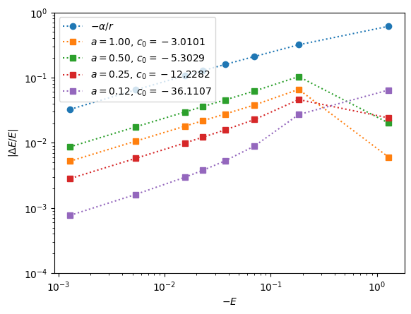
Figure 1#
Here we reproduce Fig. 1 from [Lepage, 1997] using our potential:
Show code cell content
s0 = seq.CoulombSEQ()
Es0 = np.array([s0.compute_E(_E, lam=0.999) for _E in tqdm(Es)])

fig, ax = plt.subplots()
ax.loglog(-Es, abs(Es0/Es - 1), ':o', label=r"$-\alpha/r$")
for a in [1.0, 0.5, 0.25, 0.125]:
    s1 = SEQ(a=a)
    s1.fit(Es[:1])
    Es1 = np.array([s1.compute_E(_E, lam=0.999) for _E in tqdm(Es)])
    ax.loglog(-Es, abs(Es1/Es - 1), ':s', label=f"$a={a:.2f}$, $c_0={s1.c[0]:.4f}$")
ax.legend(loc='upper left')
ax.set(ylim=(1e-4, 1), xlabel="$-E$", ylabel=r"$|\Delta E/E|$")
0%| | 0/8 [00:00<?, ?it/s]
12%|█▎ | 1/8 [00:00<00:02, 2.90it/s]
25%|██▌ | 2/8 [00:00<00:02, 2.92it/s]
38%|███▊ | 3/8 [00:01<00:01, 2.97it/s]
50%|█████ | 4/8 [00:01<00:01, 2.83it/s]
62%|██████▎ | 5/8 [00:01<00:01, 2.63it/s]
75%|███████▌ | 6/8 [00:02<00:00, 2.64it/s]
88%|████████▊ | 7/8 [00:02<00:00, 2.31it/s]
100%|██████████| 8/8 [00:03<00:00, 1.80it/s]
100%|██████████| 8/8 [00:03<00:00, 2.25it/s]
0%| | 0/1 [00:00<?, ?it/s]
100%|██████████| 1/1 [00:00<00:00, 1.50it/s]
100%|██████████| 1/1 [00:00<00:00, 1.50it/s]
0%| | 0/8 [00:00<?, ?it/s]
12%|█▎ | 1/8 [00:00<00:01, 6.47it/s]
25%|██▌ | 2/8 [00:00<00:01, 3.60it/s]
38%|███▊ | 3/8 [00:00<00:01, 3.07it/s]
50%|█████ | 4/8 [00:01<00:01, 2.89it/s]
62%|██████▎ | 5/8 [00:01<00:01, 2.59it/s]
75%|███████▌ | 6/8 [00:02<00:00, 2.33it/s]
88%|████████▊ | 7/8 [00:02<00:00, 2.08it/s]
100%|██████████| 8/8 [00:03<00:00, 1.64it/s]
100%|██████████| 8/8 [00:03<00:00, 2.15it/s]
0%| | 0/1 [00:00<?, ?it/s]
100%|██████████| 1/1 [00:00<00:00, 1.13it/s]
100%|██████████| 1/1 [00:00<00:00, 1.13it/s]
0%| | 0/8 [00:00<?, ?it/s]
12%|█▎ | 1/8 [00:00<00:01, 4.37it/s]
25%|██▌ | 2/8 [00:00<00:01, 3.29it/s]
38%|███▊ | 3/8 [00:01<00:01, 2.71it/s]
50%|█████ | 4/8 [00:01<00:01, 2.48it/s]
62%|██████▎ | 5/8 [00:02<00:01, 2.25it/s]
75%|███████▌ | 6/8 [00:02<00:00, 2.20it/s]
88%|████████▊ | 7/8 [00:03<00:00, 1.84it/s]
100%|██████████| 8/8 [00:04<00:00, 1.42it/s]
100%|██████████| 8/8 [00:04<00:00, 1.88it/s]
0%| | 0/1 [00:00<?, ?it/s]
100%|██████████| 1/1 [00:01<00:00, 1.30s/it]
100%|██████████| 1/1 [00:01<00:00, 1.30s/it]
0%| | 0/8 [00:00<?, ?it/s]
12%|█▎ | 1/8 [00:00<00:01, 3.95it/s]
25%|██▌ | 2/8 [00:00<00:01, 3.30it/s]
38%|███▊ | 3/8 [00:00<00:01, 3.06it/s]
50%|█████ | 4/8 [00:01<00:01, 3.02it/s]
62%|██████▎ | 5/8 [00:01<00:01, 2.85it/s]
75%|███████▌ | 6/8 [00:02<00:00, 2.66it/s]
88%|████████▊ | 7/8 [00:02<00:00, 2.38it/s]
100%|██████████| 8/8 [00:03<00:00, 1.93it/s]
100%|██████████| 8/8 [00:03<00:00, 2.40it/s]
0%| | 0/1 [00:00<?, ?it/s]
100%|██████████| 1/1 [00:02<00:00, 2.02s/it]
100%|██████████| 1/1 [00:02<00:00, 2.02s/it]
0%| | 0/8 [00:00<?, ?it/s]
12%|█▎ | 1/8 [00:00<00:02, 3.02it/s]
25%|██▌ | 2/8 [00:00<00:01, 3.10it/s]
38%|███▊ | 3/8 [00:00<00:01, 3.11it/s]
50%|█████ | 4/8 [00:01<00:01, 3.21it/s]
62%|██████▎ | 5/8 [00:01<00:00, 3.35it/s]
75%|███████▌ | 6/8 [00:01<00:00, 3.34it/s]
88%|████████▊ | 7/8 [00:02<00:00, 3.38it/s]
100%|██████████| 8/8 [00:02<00:00, 2.79it/s]
100%|██████████| 8/8 [00:02<00:00, 3.05it/s]
[(0.0001, 1), Text(0.5, 0, '$-E$'), Text(0, 0.5, '$|\\Delta E/E|$')]
s2 = SEQ(a=1, E_tol=1e-4)
s2.fit(Es[:2])
Es2 = np.array([s2.compute_E(_E, lam=0.999) for _E in tqdm(Es)])
0%| | 0/2 [00:00<?, ?it/s]
50%|█████ | 1/2 [00:00<00:00, 1.72it/s]
100%|██████████| 2/2 [00:07<00:00, 4.51s/it]
100%|██████████| 2/2 [00:07<00:00, 3.92s/it]
---------------------------------------------------------------------------
Exception                                 Traceback (most recent call last)
Cell In[6], line 2
      1 s2 = SEQ(a=1, E_tol=1e-4)
----> 2 s2.fit(Es[:2])
      3 Es2 = np.array([s2.compute_E(_E, lam=0.999) for _E in tqdm(Es)])

Cell In[2], line 38, in SEQ.fit(self, Es, cs, **kw)
     36 self.res = res
     37 if not res.success:
---> 38     raise Exception(res.message)
     39 self.c[:len(Es)] = res.x

Exception: The iteration is not making good progress, as measured by the
  improvement from the last five Jacobian evaluations.
s2.compute_E(Es[0]) - Es[0]
-0.01444039049322643
plt.loglog(abs(Es), abs(Es2/Es - 1))
---------------------------------------------------------------------------
NameError                                 Traceback (most recent call last)
Cell In[8], line 1
----> 1 plt.loglog(abs(Es), abs(Es2/Es - 1))

NameError: name 'Es2' is not defined