Show code cell content Hide code cell content

import mmf_setup;mmf_setup.nbinit()
import logging;logging.getLogger('matplotlib').setLevel(logging.CRITICAL)
%matplotlib inline
import numpy as np, matplotlib.pyplot as plt

$\newcommand{\vect}[1]{\mathbf{#1}} \newcommand{\uvect}[1]{\hat{#1}} \newcommand{\abs}[1]{\lvert#1\rvert} \newcommand{\norm}[1]{\lVert#1\rVert} \newcommand{\I}{\mathrm{i}} \newcommand{\ket}[1]{\left|#1\right\rangle} \newcommand{\bra}[1]{\left\langle#1\right|} \newcommand{\braket}[1]{\langle#1\rangle} \newcommand{\Braket}[1]{\left\langle#1\right\rangle} \newcommand{\op}[1]{\mathbf{#1}} \newcommand{\mat}[1]{\mathbf{#1}} \newcommand{\d}{\mathrm{d}} \newcommand{\D}[1]{\mathcal{D}[#1]\;} \newcommand{\pdiff}[3][]{\frac{\partial^{#1} #2}{\partial {#3}^{#1}}} \newcommand{\diff}[3][]{\frac{\d^{#1} #2}{\d {#3}^{#1}}} \newcommand{\ddiff}[3][]{\frac{\delta^{#1} #2}{\delta {#3}^{#1}}} \newcommand{\floor}[1]{\left\lfloor#1\right\rfloor} \newcommand{\ceil}[1]{\left\lceil#1\right\rceil} % The following allows KaTeX to render these for significantly improved % performance on CoCalc. \newcommand{\DeclareMathOperator}[2]{\newcommand{#1}{#2}} \DeclareMathOperator{\Tr}{Tr} \DeclareMathOperator{\erf}{erf} \DeclareMathOperator{\erfi}{erfi} \DeclareMathOperator{\sech}{sech} \DeclareMathOperator{\sn}{sn} \DeclareMathOperator{\cn}{cn} \DeclareMathOperator{\dn}{dn} \DeclareMathOperator{\sgn}{sgn} \DeclareMathOperator{\order}{O} \DeclareMathOperator{\diag}{diag} % \newcommand{\mylabel}[1]{\label{#1}\tag{#1}} \newcommand{\degree}{\circ}$

This cell adds /home/docs/checkouts/readthedocs.org/user_builds/physics-581-the-standard-model/checkouts/latest/src to your path, and contains some definitions for equations and some CSS for styling the notebook. If things look a bit strange, please try the following:

• Choose "Trust Notebook" from the "File" menu.
• Re-execute this cell.
• Reload the notebook.

S-Wave Scattering

A subtlety of QFT is defining “incoming” and an “outgoing” states. This generally requires having a solvable (i.e. non-interacting) theory far from the scattering potential, but in general, this is not the case. Thus, one must artificially turn the interactions on and off slowly enough to define these states without changing the physics.

In quantum mechanics, far away we simply have the free-particle Schrödinger equation, so we can use plane-wave states \(e^{\I \vect{k} \cdot \vect{r}}\). Even here we hit the issue that these “states” are not normalizable, and hence not in our Hilbert space. A careful treatment using wave packets shows that our simplified plane-wave approach is justified

The essence of scattering is to find solutions to the Schrödinger equation consisting of a superposition of an “incoming wave” and a scattered “outgoing wave”. To describe these, we need to know what the solutions to the Schrödinger equation in free space:

\[\begin{gather*} \underbrace{\left(\frac{-\hbar^2\vect{\nabla}^2}{2m} - E\right)}_{\op{H}_0} \psi(\vect{r}) = 0. \end{gather*}\]

These are simply plane waves:

\[\begin{gather*} \psi_{\vect{k}}(\vect{r}) = \braket{r|\vect{k}} = e^{\I\vect{k}\cdot\vect{r}}, \qquad E = \frac{\hbar^2 k^2}{2m}. \end{gather*}\]

Note that there is a large amount of degeneracy: all states the surface of a sphere \(\abs{\vect{k}} = k\) in momentum space have the same energy.

To describe scattering off of a small potential centered at the origin, we should express these in spherical coordinates. We expect that we should be able to arrange the degenerate plane-waves for a given energy \(E\) into specific combinations that have definite angular momentum, which is the point of spherical harmonics as we shall discuss below in section S-Wave Scattering.

Scattering Amplitude

Here \(\uvect{r} = \vect{r}/r\) is the unit vector in the \(\vect{r}\) direction. It specifies a location on the sphere, and could be replaced in spherical coordinates by \(\uvect{r} \equiv (\theta, \phi)\). Sometimes one also uses the notation \(\Omega\) in the context of \(\d{\Omega} = \sin \theta\, \d{\theta}\, \d{\phi}\) as being the solid angle.

Scattering is studied by looking for wavefunctions of the form

\[\begin{gather*} \psi(\vect{r}) = e^{\I k z} + f(k, \uvect{r})\frac{e^{\I k r}}{r} \end{gather*}\]

far from the potential. This state represents a plane-wave with energy \(E = \frac{\hbar^2k^2}{2m}\) traveling upwards along the \(z\) axis, then scattering into an outgoing wave. We will consider scattering off of a short-range potential with \(V(r>r_0) = 0\). The function \(f(k, \uvect{r})\) is called the scattering amplitude: it contains all the information about the scattering process that we can deduce from far away by looking at what is scattered from the potential. In the limit where \(kr_0 \ll 1\), we expect that \(f(k, \uvect{r}) \rightarrow f(k)\) becomes spherically symmetric – i.e. a long-wavelength probe should only see that there is small scattering site, but will not be able to resolve any details about the angular structure. This needs some justification, but holds true, and we shall use this here.

To Do: Explain this better, connecting with classical scattering.

The scattering amplitude \(f\) is complex, but has the dimensions of length. Its magnitude can be interpreted as giving the distance from the scattering potential where the flux of scattered particles equals the flux of incoming particles. Thus, the integral gives the total cross-section:

\[\begin{gather*} \sigma = \int \d{\Omega} \abs{f(k, \uvect{r})}^2 = 4\pi \abs{f(k)}^2, \end{gather*}\]

where the latter is valid in the spherically symmetric low-energy limit.

Phase Shifts

We consider the specific state \(\vect{k} = (0, 0, k)\): \(\vect{k}\vect{r} = k z = k r \cos \theta\). Recall also that integrating over the entire sphere in 3D gives:

\[\begin{gather*} 4\pi = \int \d{\Omega} = \int_{0}^{2\pi}\d{\phi}\int_{0}^{\pi} \sin \theta \d{\theta}\\ = -\int_{0}^{2\pi}\d{\phi}\int_{1}^{-1} \d{(-\cos \theta)}\\ = 2\pi\int_{-1}^{1} \d{(\cos \theta)}. \end{gather*}\]

For now we focus on S-wave scattering, considering only the spherically symmetric portions of the plane waves. To this end, we average over all angles \(\Omega \equiv (\theta, \phi) \equiv \uvect{r}\):

\[\begin{gather*} \frac{1}{4\pi}\int \d{\Omega}\; e^{\I k z} = \frac{1}{2}\int_{-1}^{1}e^{\I k r \cos\theta}\d{(\cos\theta)} = \underbrace{\frac{\sin kr}{kr}}_{\sinc kr} = \frac{1}{2\I k}\Biggl( \underbrace{\frac{e^{\I kr}}{r}}_{\text{outgoing}} - \underbrace{\frac{e^{-\I kr}}{r}}_{\text{incoming}} \Biggr). \end{gather*}\]

Here we rely on the statement above that \(f(k, \uvect{r}) \rightarrow f(k)\) in the low-energy limit. High-energy scattering off of an irregular potential can change the angular momentum of the states, allowing for a reduction (or increase) in the scattered S-wave component after averaging.

If we have a potential \(V(r)\) at the origin, then it can scatter the incoming wave, so that the outgoing wave has the form:

\[\begin{gather*} \frac{2\I k}{4\pi} \int \d{\Omega}\; \psi(\vect{r}) = \Bigl(1 + 2\I k f(k)\Bigr)\frac{e^{\I k r}}{r} - \frac{e^{-\I kr}}{r} = \frac{e^{\I (k r + 2\delta)}}{r} - \frac{e^{-\I kr}}{r}. \end{gather*}\]

In the last expression, we demand that the only effect of the potential can be to induce a phase-shift to ensure that the same incoming probability is outgoing, i.e. particles are conserved, so all incoming particles must also go out. This gives the following relationship between the phase shift \(\delta\) and the scattering amplitude \(f(k)\):

Details.

\[\begin{align*} e^{2\I\delta} &= \cos(2\delta) + \I \sin(2\delta)\\ &= \cos^2\delta - \sin^2\delta + 2\I \sin\delta\cos\delta\\ &= 1 - 2\sin^2\delta + 2\I \sin\delta\cos\delta\\ &= 1 + 2\I \sin\delta(\I\sin\delta + \cos\delta)\\ &= 1 + 2\I e^{\I\delta}\sin\delta,\\ 2\I k f(k) &= 2\I e^{\I\delta}\sin\delta,\\ f(k) &= e^{\I\delta}\frac{\sin\delta}{k}. \end{align*}\]

\[\begin{gather*} f(k) = e^{\I \delta}\frac{\sin\delta}{k}. \end{gather*}\]

Note that this implies that the total cross-section can be expressed as:

\[\begin{gather*} \sigma = 4\pi \abs{f}^2 = 4\pi \frac{\Im f}{k}. \end{gather*}\]

This is a consequence of the optical theorem which relates the total number of scattered particles to the loss of scattered particles in the forward direction. (The optical theorem is written in terms of forward scattering amplitude \(\Im f(\theta=0)\), but here \(f\) is independent of the angle, so \(f(\theta=0) = f\).)

This form also explains why we introduced a phase shift of \(2\delta\) in the outgoing wave. Consider the radial wavefunction \(u(r) = r\psi(r)\). In this picture, we have an incoming plane wave \(-e^{-\I kr}\) scattering into a phase-shifted outgoing wave \(e^{\I (kr + 2\delta)}\):

\[\begin{gather*} u(r) \xrightarrow[r \rightarrow \infty]{} e^{\I(kr + 2\delta)} - e^{-\I kr} = 2\I e^{\I\delta}\frac{e^{\I(kr + \delta)} - e^{-\I (kr + \delta)}}{2\I} = 2\I e^{\I\delta}\sin(kr + \delta). \end{gather*}\]

(Remember that multiplying a wavefunction by an overall phase or constant does not affect the physics. Thus, the factor of \(2\I e^{\I\delta}\) is physically inconsequential.) Thus, the scattering results in an interference pattern that is phase-shifted by \(\delta\) from the interference pattern obtained with no potential.

Calculating the phase shift \(\delta\).

This interference can be used to determine the relationship between the S-wave phase shift \(\delta\) and the energy \(E\) using a slight trick. Place the potential \(V(r)\) at the center of a large spherical box of radius \(R\) such that the radial wavefunction satisfies

\[\begin{gather*} \left( \frac{-\hbar^2}{2m}\diff[2]{}{r} - V(r) \right)u(r) = Eu(r), \qquad u(0) = u(R) = 0. \end{gather*}\]

Solutions to this BVP outside of the range of the potential will have the form of the interference pattern \(\sin(kr + \delta)\) with the boundary condition \(u(R) = 0\) so that

\[\begin{gather*} kR + \delta = n\pi. \end{gather*}\]

Extending this solution beyond \(R\) gives a solution to the S-wave scattering problem with precisely the same relationship between \(\delta\) and \(E = \hbar^2 k^2/2m\) for this potential.

Scattering Length

\[\begin{gather*} \Im f = \frac{\sin^2 \delta}{k} = k\abs{f}^2 \end{gather*}\]

The normalization follows from

\[\begin{align*} \psi(r) &= A \frac{e^{-\kappa r}}{r},\\ 1 &= \int\d^3{\vect{r}}\abs{\psi(\vect{r})}^2\\ &= 4\pi A^2 \int_0^{\infty}\d{r}\; r^2e^{-2\kappa r} \\ &= \frac{\pi A^2}{\kappa^3} \end{align*}\]

Consider bound states of a short-range potential \(V(r>r_0)=0\). Beyond \(r_0\) the radial wavefunction must be

\[\begin{gather*} u(r>r_0) = Ae^{-\kappa r}, \qquad \kappa = \sqrt{-2mE}. \end{gather*}\]

Note that this solution remains finite if one takes \(r_0 \rightarrow 0\) while simultaneously adjusting the depth of the potential to maintain a fixed energy \(E<0\). Thus, we can write \(\psi(r) = Ae^{-\kappa r}/r\) and integrate to obtain the normalized wavefunction

\[\begin{gather*} \psi(r) = \sqrt{\frac{\kappa^3}{\pi}}\frac{e^{-\kappa r}}{r} \rightarrow \sqrt{\frac{\kappa^3}{\pi}}\left(\frac{1}{r} - \kappa + \dots\right), \qquad u(r) \rightarrow \sqrt{\frac{\kappa^3}{\pi}}(1 - \kappa r + \dots) \end{gather*}\]

Note that we have not specified any details about the form of \(V(r)\) other than it having a short range and a fixed bound state \(E\). This is a key point of effective theories: low energy physics should be universal, and largely independent of short-distance structure of the potential.

We have expanded these in the low-energy limit \(\kappa \rightarrow 0\), and see that the radial wavefunction becomes linear, intersecting the axis at \(r=1/\kappa\). It turns out that this is the S-wave scattering length:

\[\begin{gather*} a = \frac{ \end{gather*}\]

Incomplete…

This can be codified in some sort of local pseudo-potential with that enforces the condition

\[\begin{gather*} \lim_{r\rightarrow 0} \Bigl(u'(r) + \kappa u(r)\Bigr) = 0. \end{gather*}\]

What is the form of this pseudo-potential? One often sees \(V(\vect{r}) = c\delta^{3}(\vect{r})\), but as [Lepage, 1997] points out (c.f. Eqs. (4) and (6) and the following discussion) , the delta-function is too singular.

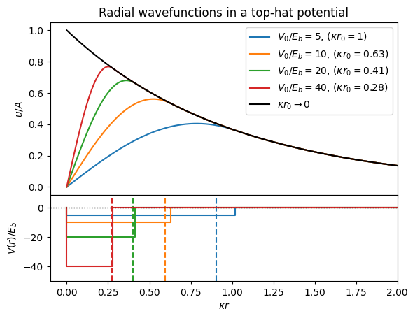
Example: Top-Hat Potential

To see this, consider an explicit realization of a top-hap potential \(V(r) = -V_0\Theta(r_0-r)\) with depth \(-V_0\) and range \(r_0\). The bound-states \(E = -E_b\) of the radial wavefunction have the following solutions

Here we use

\[\begin{gather*} \frac{\hbar^2k^2}{2m} - V_0 = \frac{-\hbar^2 \kappa^2}{2m} = -E_b, \end{gather*}\]

and the fact that both \(u(r)\) and \(u'(r)\) must be continuous at \(r_0\). We also note that \(kr_0 > \pi/2\) so let \(kr_0 = \tfrac{\pi}{2} + \alpha\) and use \(\cot(\tfrac{1}{2}\pi + \alpha) = -\tan(\alpha)\).

\[\begin{gather*} u(r) = \begin{cases} B\sin(k r) & r < r_0,\\ Ae^{-\kappa r} & r>r_0, \end{cases} \qquad \hbar \kappa = \sqrt{2mE_b}, \qquad \hbar k = \sqrt{2m(V_0 - E_b)},\\ B\sin(kr_0) = Ae^{-\kappa r_0}, \qquad kB\cos(kr_0) = -\kappa Ae^{-\kappa r_0}. \end{gather*}\]

Combining these, we have the transcendental equation.

\[\begin{gather*} \hbar k\cot(kr_0) = -\hbar k\tan(k r_0 - \tfrac{\pi}{2}) = -\hbar \kappa = -\sqrt{2mE_b},\\ kr_0 = \frac{\pi}{2} + \cot^{-1}\sqrt{\frac{V_0}{E_b}-1}. \end{gather*}\]

Taking \(V_0 \rightarrow \infty\), we can expand this to obtain the limiting behaviour in the short-range limit for fixed binding energy \(E_b\):

\[\begin{gather*} kr_0 = \frac{\pi}{2} + \sqrt{\frac{E_b}{V_0}} + \frac{1}{6}\sqrt{\frac{E_b}{V_0}}^3 + O(E_b/V_0)^5/2,\\ r_0 \rightarrow \frac{\pi}{2k} \approx \frac{\pi \hbar}{\sqrt{8mV_0}}\left( 1 + \frac{2}{\pi}\sqrt{\frac{E_b}{V_0}} + O\left(\frac{E_b}{V_0}\right) \right)\\ V_0 \rightarrow \frac{m\hbar^2}{2 r_0^2} \left( \pi^2 + 8\kappa r_0 + O(\kappa r_0)^2 \right). \end{gather*}\]

Details

Let \(x = E_b/V_0 \rightarrow 0\).

\[\begin{gather*} \cot^{-1} \sqrt{1/x - 1} = \sqrt{x} + \frac{x^{3/2}}{6} + O(x^{5/2})\\ \frac{1}{\sqrt{1-x}} = 1 + \frac{x}{2} + O(x^2)\\ \frac{\sqrt{2mV_0}}{\hbar}r_0 = \frac{\frac{\pi}{2} + \cot^{-1}\sqrt{1/x - 1}}{\sqrt{1-x}}\\ = \frac{\pi}{2} + \sqrt{x} + \frac{\pi}{4}x + \frac{2}{3}x^{3/2} + O(x^2)\\ = \frac{\pi}{2}\left(1 + \frac{2}{\pi}\sqrt{x} + \frac{1}{2}x + \frac{4}{3\pi}x^{3/2} + O(x^2)\right),\\ \frac{2}{\pi}\kappa r_0 = y = \sqrt{x} + \frac{2}{\pi}\sqrt{x}^2 + \frac{1}{2}\sqrt{x}^{3} + \frac{4}{3\pi}\sqrt{x}^{4} + O(\sqrt{x}^{5}),\\ \end{gather*}\]

We can then use the series reversion formula to compute

\[\begin{gather*} y = \sqrt{x} + a_2 \sqrt{x}^2 + a_3 \sqrt{x}^3 + \dots\\ \sqrt{x} = y + A_2y^2 + A_3y^3 + \cdots\\ \sqrt{x} = y - a_2y^2 + (2a_2^2 - a_3)y^3 + \dots = y - \frac{2}{\pi}y^2 + \left(\frac{8}{\pi^2} - \frac{1}{2}\right)y^3 + \dots. \end{gather*}\]

Then we have

\[\begin{gather*} V_0 = \frac{E_b}{x} = \frac{E_b}{(y+A_2y^2 + A_3y^3)^2} = \frac{E_b}{y^2(1+A_2y + A_3y^2)^2}\\ = \frac{E_b}{y^2}\left(1 - 2 A_2 y + (3A_2 - 2A_3)y^2 + (6A_2A_3 - 4A_2^3)y^3 + \cdots\right)\\ = \frac{E_b}{y^2}\left( 1 + \frac{4}{\pi} y + (1 - \tfrac{6}{\pi} - \tfrac{16}{\pi^2})y^2 + (\tfrac{6}{\pi} - \tfrac{64}{\pi^3})y^3 + \cdots\right)\\ = \frac{m\hbar^2 \kappa^2 \pi^2}{2\kappa^2 r_0^2} \left( 1 + \frac{8}{\pi^2}\kappa r_0 + (1 - \tfrac{6}{\pi} - \tfrac{16}{\pi^2})\tfrac{4}{\pi^2}(\kappa r_0)^2 + (\tfrac{6}{\pi} - \tfrac{64}{\pi^3})\tfrac{8}{\pi^3}(\kappa r_0)^3 + \cdots\right). \end{gather*}\]

Note: There is something wrong here with the higher order terms. Leading order works out.

The point of Shina Tan’s work [Tan, 2005] is introduce generalized delta-like “selectors” \(\lambda(\vect{r})\) and \(l(\vect{r})\) that are zero everywhere except \(\vect{r}=0\) and satisfy

\[\begin{gather*} \int \d^3{\vect{r}} \Bigl(a\lambda(\vect{r}) + b l(\vect{r})\Bigr) = a,\\ \int \d^3{\vect{r}} \Bigl(a\tfrac{\lambda(\vect{r})}{4\pi r} + b\tfrac{l(\vect{r})}{4\pi r}\Bigr) = b,\\ \int \d^3{\vect{r}} \Bigl(a\uvect{r}\lambda(\vect{r}) + b \uvect{r}l(\vect{r})\Bigr) = 0. \end{gather*}\]

These can be used to rigorously construct appropriate pseudo-potentials.

Note that this is a very peculiar limiting behaviour. The leading order behaviour has constant \(V_0 \propto 1/r_0^2\) which is independent of the binding energy \(E_b = \hbar^2\kappa^2/2m\). This is a two-dimensional delta-function: more singular than a single delta-function, but not as singular as the 3D delta-function discussed in [Lepage, 1997]. Thus, in order to specify the universal low-energy behaviour of short-range potentials, one needs a special type of pseudo-potential that can be constructed using selectors [Tan, 2005].

We can understand the effect here in two steps:

1. The second order term has constant \(V_0 r_0\): this is a delta-function in 1D, and can give the kink in the wavefunction that develops as we take \(r_0 \rightarrow 0\). However, representing the potential for \(u(r)\) as \(c\delta(r)\) by itself should have no effect since the radial wavefunction \(u(0) = 0\) vanishes.

2. Thus, we need something even stronger to “kick” \(u(0)\) to a finite value before the delta-function above can be used to specify the magnitude of the kink, and therefore fix the energy. This is the leading order piece with \(V_0 r_0^2\) that is independent of \(\kappa\) and \(E_b\).

This is why Tan needs a combination of two selectors [Tan, 2005].

Show code cell source Hide code cell source

hbar = 1
m = 0.5
Eb = 1
kappa = np.sqrt(2*m*Eb)
A = np.sqrt(kappa**3/np.pi)
R = 2.0
r = np.linspace(0, R, 1000)
u0 = A*np.exp(-kappa*r)

fig, axs = plt.subplots(2, 1, sharex=True, height_ratios=(2, 1), gridspec_kw=dict(hspace=0))
ax, axr = axs

V0_Es = [5, 10, 20, 40]
for V0_E in V0_Es:
    V0 = V0_E * Eb
    k = np.sqrt(2*m*(V0 - Eb))
    r0 = (np.pi/2 + np.arctan(1/np.sqrt(V0/Eb - 1)))/k
    r0_ = np.pi*hbar /np.sqrt(8*m*V0)*(1 + 2/np.pi*np.sqrt(Eb/V0))  # Limiting approximation
    y = V0/(m*hbar**2*np.pi**2/2/r0**2)
    c1 = 8/np.pi**2
    c2 = (1- 6/np.pi - 16/np.pi**2)*4/np.pi**2  # This is wrong, it should be about 0.24103
    #print(y, 
    #      (y - 1)/(c1*kappa*r0), 
    #      (y - 1 - c1*kappa*r0)/((kappa*r0)**2))
    B = A*np.exp(-kappa*r0)/np.sin(k*r0)
    u = np.where(r<r0, B*np.sin(k*r), u0)
    l, = ax.plot(kappa*r, u/A, label=fr"$V_0/E_b={V0_E}$, ($\kappa r_0={kappa*r0:.2g}$)")
    axr.plot([0, 0, kappa*r0, kappa*r0, R], [0, -V0, -V0, 0, 0], '-', c=l.get_c())
    axr.axvline(kappa*r0_, c=l.get_c(), ls="--")
axr.axhline(0, c='k', ls=':', lw=1)
ax.plot(kappa*r, u0/A, '-k', label=r"$\kappa r_0\rightarrow 0$")
ax.set(xlim=(-0.1, 2.0), ylabel="$u/A$", 
       title="Radial wavefunctions in a top-hat potential")
axr.set(ylim=(-50, 9), xlabel="$\kappa r$", ylabel="$V(r)/E_b$")
ax.legend();

1D Scattering

This requirement can be loosened to requiring

\[\begin{gather*} \int_{-\infty}^{\infty}\d{x}(1+x^2)V(x) < \infty. \end{gather*}\]

For a different perspective, we now consider scattering in 1D. We consider scattering of a state with energy \(E_k\) off of a potential \(V(x)\) that has compact support \(\abs{x} < R\) about the origin. (I.e. \(V(x) = 0\) for \(\abs{x}>R\).) We then write

\[\begin{gather*} E_k = \frac{\hbar^2k^2}{2m}, \qquad \psi(x) = \begin{cases} t_k e^{-\I k x} & x < -R, \\ e^{-\I k x} + r_k e^{\I k x} & x > R. \end{cases} \end{gather*}\]

This corresponds to an incoming plane wave with momentum \(-k\) reflecting off the barrier with reflection amplitude \(r_k\) and transmission amplitude \(t_k\). Conservation of probability requires

\[\begin{gather*} \abs{r_k}^2 + \abs{t_k}^2 = 1. \end{gather*}\]

In addition to the scattering states, the potential may support a finite number of bound states with energy

\[\begin{gather*} E_n = - \frac{\hbar^2 \kappa_n^2}{2m}, \qquad \psi_n(x) = \begin{cases} d_{n}e^{\kappa_n x} & x < -R,\\ c_{n}e^{-\kappa_n x} & x > R, \end{cases}, \qquad \int_{-\infty}^{\infty}\d{x}\; \abs{\psi(x)}^2 = 1. \end{gather*}\]

This scattering data – \([r_k, t_k, c_n, \kappa_n]\) – can be collected into a single function

\[\begin{gather*} F(x) = \int \frac{\d{k}}{2\pi} r_k e^{\I k x} + \sum_{n} c_n^2 e^{-\kappa_n x}. \end{gather*}\]

Apparently, solving the Gelfand-Levitan-Marchenko (GLM) equation allows one to reconstruct the potential

\[\begin{gather*} K(x, y) + F(x+y) + \int_x^{\infty} K(x, z)F(z+y)\d{z} = 0,\\ V(x) = -2\diff{K(x, x)}{x}. \end{gather*}\]

\[\begin{gather*} K(x, y) + F(x+y) + \int_x^{\infty} K(x, z)F(z+y)\d{z} = 0,\\ K_{,x}(x, y) + F'(x+y) - K(x, x)F(x+y) + \int_x^{\infty} K_{,x}(x, z)F(z+y)\d{z} = 0\\ K_{,y}(x, y) + F'(x+y) + \int_x^{\infty} K(x, z)F'(z+y)\d{z} = 0\\ F'(x) = \int \frac{\d{k}}{2\pi} \I k r_k e^{\I k x} - \sum_{n} \kappa_n c_n^2 e^{-\kappa_n x},\\ \diff{K(x, x)}{x} = -2F'(2x) + K(x, x)F(2x) - \int_x^{\infty} [K(x, z) + K_{,x}(x, z)]F(z+x)\d{z}. \end{gather*}\]

General Scattering

Recall that the Schrödinger equation has the following form in spherical coordinates:

\[\begin{align*} \psi_{nlm}(r) &= \psi_{r}(r)Y_{l}^{m}(\theta, \phi),\\ \frac{1}{r^2}\diff{}{r}\left(r^2\diff{\psi_r(r)}{r}\right) - \frac{l(l+1)}{r^2}\psi_r(r) &= \frac{2m}{\hbar^2}\bigl(V(r) - E\bigr)\psi_r(r),\\ \left( \diff[2]{}{r} - \frac{2}{r}\diff{}{r} + \frac{l(l+1)}{r^2}\right)\psi_r(r) &= \frac{2m}{\hbar^2}\bigl(V(r) - E\bigr)\psi_r(r), \end{align*}\]

Show code cell source Hide code cell source

from scipy.special import spherical_jn, spherical_yn

kr = np.linspace(0, 20, 1000)
fig, ax = plt.subplots(figsize=(4,3))
for l in range(3):
    ax.plot(kr, spherical_jn(l, kr), f"C{l}-", label=f"$j_{l}(kr)$")
for l in range(3):
    ax.plot(kr, spherical_yn(l, kr), f"C{l}--", label=f"$y_{l}(kr)$")
ax.set(xlabel="$kr$", ylim=(-0.5, 1.1), title="Spherical Bessel functions",
       yticks=[-0.5, 0, 0.5, 1])
ax.legend(loc='upper right', ncol=2)
plt.tight_layout()

or, introducing the radial wavefunction \(u(r) = r\psi_r(r)\),

\[\begin{gather*} \left(\diff[2]{}{r} - \frac{l(l+1)}{r^2}\right)u_{nl}(r) = \frac{2m}{\hbar^2}\bigl(V(r) - E\bigr) u_{nl}(r). \end{gather*}\]

Spherical Bessel functions

The spherical Bessel functions are

\[\begin{align*} j_n(x) &= +(-x)^n\left(\frac{1}{x}\diff{}{x}\right)^{n}\frac{\sin x}{x} \xrightarrow[x \rightarrow \infty]{}\frac{+\sin(x - \tfrac{\pi}{2}n)}{x} ,\\ y_n(x) &= -(-x)^n\left(\frac{1}{x}\diff{}{x}\right)^{n}\frac{\cos x}{x} \xrightarrow[x \rightarrow \infty]{}\frac{-\cos(x - \tfrac{\pi}{2}n)}{x}. \end{align*}\]

Strictly speaking, we need \(rV(r) \rightarrow 0\) as \(r \rightarrow \infty\). Note that this famously excludes the Coulomb potential, which is “long ranged” and has infinite cross-section.

Far from the potential where \(V(r) \approx 0\), this can be expressed in terms of the spherical Bessel functions \(j_{l}(kr)\) and \(y_{l}(kr)\):

\[\begin{gather*} \psi(\vect{r}) = \sum_{lm} \Bigl( A_{lm} j_{l}(kr) + B_{lm} y_{l}(kr) \Bigr) Y^{m}_{l}(\theta, \phi). \end{gather*}\]

Using the asymptotic forms, this becomes

\[\begin{gather*} \psi(\vect{r}) \xrightarrow[r \rightarrow \infty]{} \sum_{lm} \Bigl( A_{lm} \frac{\sin(kr - \tfrac{\pi}{2}l)}{kr} - B_{lm} \frac{\cos(kr - \tfrac{\pi}{2}l)}{kr} \Bigr) Y^{m}_{l}(\theta, \phi). \end{gather*}\]

An outgoing (scattered) wave should have the form \(e^{\I kr}/kr\), and therefor must have \(A_{lm} = -\I B_{lm}\):

\[\begin{gather*} \psi_{sc}(\vect{r}) \xrightarrow[r \rightarrow \infty]{} \frac{e^{\I kr}}{r} \underbrace{ \frac{1}{k} \sum_{lm} \overbrace{(-\I)^{l}}^{e^{-\I\pi l/2}} A_{lm} Y^{m}_{l}(\theta, \phi) }_{f(\theta, \phi)} = \frac{e^{\I kr}}{r}f(\theta, \phi). \end{gather*}\]

The full scattering problem can thus be expressed as

\[\begin{gather*} \psi(\vect{r}) \xrightarrow[r \rightarrow \infty]{} e^{\I k z} + f(\theta, \phi)\frac{e^{\I kr}}{r}. \end{gather*}\]

See Also

• Physics 555: Bound States in the 1D Schrödinger Equation