Notes

Notes#

[Donoghue and Sorbo, 2022] and Zee use the same metric convention.
[Donoghue and Sorbo, 2022] does not clearly/quickly present the tachyonic modes of a photon… Show this as a motivation for Gauge invariance.
Physics backgrounds will vary. Need to pair up.
Zee’s baby problem is great and we should do it, but we should include the fact that it is an asymptotic series.

Prerequisites#

Notations#

Economy of notation is important in order to simplify calculations. In physics, we need to take many derivatives, so we use various shorthand notation. You might see the following:

\[\begin{gather*} \pdiff{f(\vect{x}, t)}{x_i} = \partial_{x_i}f = f_{,x_i} = \left[\pdiff{f(\vect{x}, t)}{\vect{x}}\right]_i = [\partial_{\vect{x}} f]_{i} = [\vect{\nabla} f]_{i},\\ \pdiff{f(\vect{x}, t)}{t} = \partial_{t}f = f_{,t} = \dot{f}. \end{gather*}\]

Sometimes, when it is clear, we might use \(f' = \partial_{x}f\) for the spatial derivative in 1D.

The Laplacian is sometimes written

\[\begin{gather*} ◻︎ = ∆ = \nabla^2 = \vect{\nabla}\cdot\vect{\nabla}. \end{gather*}\]

Relativity#

We take the Minkowski metric to be \(g_{\mu\nu} = \diag(1, -1, -1, -1)\). This is the convention of [Donoghue and Sorbo, 2022] and [Zee, 2010]. Note that [`t Hooft, 2016] uses the opposite convention \(g_{\mu\nu} = \diag(-1, 1, 1, 1)\).

Principle of Extremal Action#

In classical mechanics, Newton’s law

\[\begin{gather*} m\ddot{x}(t) = F(x, t) = -V_{,x}(x, t) \end{gather*}\]

for conservative forces (those that can be expressed as the gradient of a potential function \(\vect{F} = -\vect{\nabla}V(\vect{x}, t)\) as shown) can be derived from a variational principle in terms of the action functional \(S[x]\):

\[\begin{gather*} S[x] = \int_{t_i}^{t_f}\d{t}\;L(x, \dot{x}, t), \qquad L(x, \dot{x}, t) = \frac{m\dot{x}^2}{2} - V(x, t). \end{gather*}\]

Do It!#

Show that Newton’s law follows from the condition of extremal action

\[\begin{gather*} \delta S[x] = 0 \implies \underbrace{\diff{}{t}\pdiff{L[x, \dot{x}, t]}{\dot{x}}}_{m\ddot{x}} = \underbrace{\pdiff{L[x, \dot{x}, t]}{x}}_{-\partial_{x}V(x, t)} \end{gather*}\]

where \(\delta S[x]\) is a functional derivative. I.e. solutions to Newton’s law \(x=q(t)\) that satisfy the boundary conditions \(q(t_i) = x_i\) and \(q(t_f) = x_f\) satisfy:

\[\begin{gather*} S[q(t) + \lambda \delta(t)] = S[q] + O(\lambda^2) \end{gather*}\]

for small \(\lambda\) and all deviations \(\delta(t)\) that preserve the boundary conditions \(\delta(t_i) = \delta(t_f) = 0\).

Example#

Consider a particle falling in a gravitational potential \(V = mgh\) where \(m\) is the mass of the particle and \(g\) is the acceleration due to gravity. Newton’s law

\[\begin{gather*} m\ddot{h}(t) = -mgh(t) \end{gather*}\]

has the general solution, where \(h_0 = h(0)\) and \(v_0 = h'(0)\):

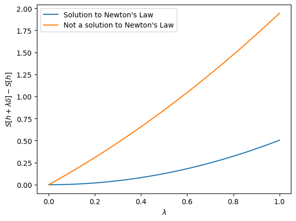
\[\begin{gather*} h(t) = h_0 + v_0t - \frac{gt^2}{2}. \end{gather*}\]

Here we demonstrate numerically that the action is indeed quadratic in \(\lambda\) for the solution to Newton’s law, but that something that is not a solution to Newton’s law has a linear dependence on \(\lambda\).

m = 1.2
g = 9.8
h0 = 10.1
v0 = 2.3
t0 = 0
tf = np.sqrt(h0/g)

t = np.linspace(t0, tf, 1000)
h = h0 + v0*t - g*t**2/2
dh_dt = v0 - g*t

h_wrong = h0 + v0*t - g*t**2/2  # Wrong!  (factor in denomonator)
dh_wrong_dt = v0 - g*t/2

# Put whatever you like here, but keep the prefactor
delta = (t-t0)*(t-tf)*np.exp(t**2)
ddelta_dt = np.gradient(delta, t, edge_order=2)

def get_S(h, dh_dt):
    L = m*dh_dt**2/2 - m*g*h
    return np.trapz(L, t)

lams = np.linspace(0, 1)
Ss = [get_S(h+lam*delta, dh_dt + lam*ddelta_dt) for lam in lams]
Ss_wrong = [get_S(h_wrong+lam*delta, dh_wrong_dt + lam*ddelta_dt) for lam in lams]
fig, ax = plt.subplots()
ax.plot(lams, Ss-Ss[0], label="Solution to Newton's Law")
ax.plot(lams, Ss_wrong-Ss_wrong[0], label="Not a solution to Newton's Law")
ax.legend()
ax.set(xlabel="$\lambda$", ylabel=r"$S[h+\lambda\delta] - S[h]$");

../_images/59dd1ccc9c19e99a4169b5258724e791d074aae5a4d61b29fa92d6ba6dbd77ac.png

Quantum Mechanics#

Please review the solution of a harmonic oscillator (HO) in quantum mechanics

\[\begin{gather*} \op{H} = \frac{\hbar^2}{2m}\op{p}^2 + \frac{m\omega^2}{2}\op{x}^2, \qquad [\op{x}, \op{p}] = \I \hbar, \end{gather*}\]

so that you are comfortable with the notation of raising and lowering operators

\[\begin{gather*} \op{a} = \sqrt{\frac{m\omega}{2\hbar}}\op{x} + \I \sqrt{\frac{1}{2m\omega \hbar}}\op{p},\\ \op{a}^\dagger = \sqrt{\frac{m\omega}{2\hbar}}\op{x} - \I \sqrt{\frac{1}{2m\omega \hbar}}\op{p},\\ [\op{a}, \op{a}^\dagger] = 1. \end{gather*}\]

These allow us to factor the Hamiltonian

\[\begin{gather*} \op{H} = \hbar\omega \left(\op{a}^\dagger \op{a} + \frac{1}{2}\right), \qquad \op{H}\ket{n} = \ket{n}E_n, \qquad E_n = \hbar\omega(n + \tfrac{1}{2}), \end{gather*}\]

and construct eigenstates \(\ket{n}\) from the ground state \(\ket{0}\) where \(\op{a}\ket{0} = 0\):

\[\begin{gather*} \op{a}^\dagger\ket{n} = \sqrt{n+1}\ket{n+1}, \qquad \op{a}\ket{n+1} = \sqrt{n+1}\ket{n}. \end{gather*}\]

In quantum field theory the analog of the operator \(\op{n} = \op{a}^\dagger\op{a}\) (which has eigenvalues \(n\) here) will count the number of quanta in a state.

Phonons#

Classical Theory#

Following the text [Donoghue and Sorbo, 2022], we work out the theory here for phonons on a string of masses and springs.