Show code cell content Hide code cell content

import mmf_setup;mmf_setup.nbinit()
import logging;logging.getLogger('matplotlib').setLevel(logging.CRITICAL)
%matplotlib inline
import numpy as np, matplotlib.pyplot as plt

$\newcommand{\vect}[1]{\mathbf{#1}} \newcommand{\uvect}[1]{\hat{#1}} \newcommand{\abs}[1]{\lvert#1\rvert} \newcommand{\norm}[1]{\lVert#1\rVert} \newcommand{\I}{\mathrm{i}} \newcommand{\ket}[1]{\left|#1\right\rangle} \newcommand{\bra}[1]{\left\langle#1\right|} \newcommand{\braket}[1]{\langle#1\rangle} \newcommand{\Braket}[1]{\left\langle#1\right\rangle} \newcommand{\op}[1]{\mathbf{#1}} \newcommand{\mat}[1]{\mathbf{#1}} \newcommand{\d}{\mathrm{d}} \newcommand{\D}[1]{\mathcal{D}[#1]\;} \newcommand{\pdiff}[3][]{\frac{\partial^{#1} #2}{\partial {#3}^{#1}}} \newcommand{\diff}[3][]{\frac{\d^{#1} #2}{\d {#3}^{#1}}} \newcommand{\ddiff}[3][]{\frac{\delta^{#1} #2}{\delta {#3}^{#1}}} \newcommand{\floor}[1]{\left\lfloor#1\right\rfloor} \newcommand{\ceil}[1]{\left\lceil#1\right\rceil} % The following allows KaTeX to render these for significantly improved % performance on CoCalc. \newcommand{\DeclareMathOperator}[2]{\newcommand{#1}{#2}} \DeclareMathOperator{\Tr}{Tr} \DeclareMathOperator{\erf}{erf} \DeclareMathOperator{\erfi}{erfi} \DeclareMathOperator{\sech}{sech} \DeclareMathOperator{\sn}{sn} \DeclareMathOperator{\cn}{cn} \DeclareMathOperator{\dn}{dn} \DeclareMathOperator{\sgn}{sgn} \DeclareMathOperator{\order}{O} \DeclareMathOperator{\diag}{diag} % \newcommand{\mylabel}[1]{\label{#1}\tag{#1}} \newcommand{\degree}{\circ}$

This cell adds /home/docs/checkouts/readthedocs.org/user_builds/physics-581-the-standard-model/checkouts/latest/src to your path, and contains some definitions for equations and some CSS for styling the notebook. If things look a bit strange, please try the following:

• Choose "Trust Notebook" from the "File" menu.
• Re-execute this cell.
• Reload the notebook.

How to Solve the (Radial) Schrödinger Equation

Here we show how to accurately solve the radial Schrödinger equation numerically with long-range Coulomb potential:

\[\begin{gather*} \left( \frac{\hbar^2}{2m} \left(-\diff[2]{}{r} + \frac{\nu^2 - 1/4}{r^2}\right) + V(r)\right) u(r) = E u(r),\\ u(r) = r^{(d-1)/2}\psi(r), \qquad \nu = l + \frac{d}{2} - 1, \end{gather*}\]

where \(V(r) \rightarrow -\alpha/r\) for large \(r\).

For now, we restrict our attention to \(d=3\) dimensions, and \(S\)-wave states where \(l=0\) so that \(\nu^2 - 1/4 = 0\). The radial wavefunctions \(u(r)\) thus satisfy a 1D Schrödinger equation:

\[\begin{gather*} \braket{r|\op{H}|u} = \underbrace{ \left(\frac{-\hbar^2}{2m}\diff[2]{}{r} + V(r)\right) }_{\op{H}} \underbrace{u(r)}_{\ket{u}} = E u(r), \qquad u(0) = 0, \qquad u(\infty) = 0. \end{gather*}\]

Since the operator is linear, this is formally an eigenvalue problem in function space:

\[\begin{gather*} \op{H}\ket{u} = \ket{u}E. \end{gather*}\]

Strategies

There are two basic strategies for solving this type of problem: Shooting and diagonalization. The first is to solve an initial value problem (IVP) with a high-precision solver, and then use a root-finder to adjust the eigenvalue \(E\) so that the solution converges to the appropriate boundary condition. The second involves finding a matrix approximation for the Hamiltonian \(\op{H}\) and diagonalizing this matrix. Each method has its pros and cons:

Shooting

• (+) Conceptually simple and capable of high accuracy.

• (+) Can use high-precision adaptive integrates like scipy.integrate.solve_ivp() in combination with robust root-finders like scipy.optimize.brentq().

• (-) Need to shoot for each eigenstate.

• (-) Must determine bounds for the energies. This can require extensive book-keeping or clever searching strategies to ensure states are not missed.

• (-) Exponentially growing solutions can break numerically.

• (-) Can’t shoot from singular points, and can’t shoot to \(\infty\) without complications.

Some of these negatives can be compensated for by changing variables, or shooting from interior points.

Diagonalization

• (+) Simple if you know the right basis.

• (+) Returns all eigenstates and energies at once.

• (+) Can be simple and sometimes accurate if the right basis can be found (esp. if the problem is analytic and spectral methods can be used).

• (-) Not highly accurate if the problem is not analytic or a good basis cannot be found.

We start by demonstrating the diagonalization approach with finite differences since it is very easy to implement and works extremely well in some cases. Unfortunately, to do well with Coulomb-like potentials requires finding a good basis, and this is not trivial, so our ultimate strategy will rely on shooting for finding highly accurate solution.

TL;DR Teaser

As a teaser and to show you how these can work well, we solve the problem of a 1D harmonic oscillator:

\[\begin{gather*} \frac{-\hbar^2}{2m}\psi''(x) + \frac{m\omega^2x^2}{2}\psi(x) = E\psi(x), \qquad \psi(\pm \infty) = 0, \qquad E_n = \hbar \omega (n + \tfrac{1}{2}). \end{gather*}\]

We give no discussion here, but choose fairly optimal parameters to find the solutions for the first 20 states to machine precision.

Diagonalization

hbar = m = w = 1
N = 64
L = 20.0
a = dx = L/N
n = np.arange(N)
x = n*dx - L//2
a_ho = np.sqrt(hbar/m/w)
N_states = 20

Vx = m*(w*x)**2/2
En = hbar*w*(np.arange(N) + 0.5)  # Exact solutions

# Fourier Basis
k = 2*np.pi * np.fft.fftfreq(N, a)
K = np.fft.ifft(hbar**2*k**2/2/m * np.fft.fft(np.eye(N), axis=1), axis=1)
V = np.diag(Vx)
Es, psis = np.linalg.eigh(K+V)
print(f"Max Relative error = {abs((Es/En-1)[:N_states]).max()} for {N_states} states.")

Max Relative error = 1.8540724511240114e-14 for 20 states.

Show code cell source Hide code cell source

fig, ax = plt.subplots(figsize=(5,6))
ax.plot(x/a_ho, Vx / (hbar * w), '-b')
for n in range(N_states):
    E, psi = Es[n], psis[:, n]
    i = np.argmax(abs(psi))
    psi /= psi[i]  # Normalize and make real
    assert np.allclose(psi.imag, 0)
    psi = psi.real
    x0 = np.sqrt(2*E/m)/w
    l, = ax.plot(x/a_ho, E + 0.4*psi, '.-', ms=1, lw=0.5, label=f"$E_{{{n}}}$")
    l = ax.axhline(E, ls='--', c=l.get_c(), lw=0.5)
    
ax.set(xlim=(-x0-1, x0+1), ylim=(-1, N_states + 1), 
       xlabel="$x/a_{HO}$", ylabel="$E$ ($ + \epsilon \psi(x)$)");

This demonstrates the power of a carefully-tuned spectral methods: with only 64 points, we have machine precision for the 20 lowest states in less than 20 lines of code (including printing, checks, etc.)

For fun, let’s see how \(E\) depends on an anisotropy:

\[\begin{gather*} V(x) = \frac{m\omega^2x^2}{2} + \epsilon x^4. \end{gather*}\]

I encourage you to compare these results to what you get from perturbation theory. Do you expect perturbation theory to converge?

Show code cell source Hide code cell source

N = 64*2  # Need more points for convergence.  Why?
L = 20.0
a = dx = L/N
n = np.arange(N)
x = n*dx - L//2
k = 2*np.pi * np.fft.fftfreq(N, a)
K = np.fft.ifft(hbar**2*k**2/2/m * np.fft.fft(np.eye(N), axis=1), axis=1)

epss = np.linspace(0, 1, 100)

Es = []
for eps in epss:
    Vx = m*(w*x)**2/2 + eps*x**4
    V = np.diag(Vx)
    Es.append(np.linalg.eigvalsh(K+V)[:N_states])
    
Es = np.asarray(Es)
fig, ax = plt.subplots(figsize=(4,3))
ax.plot(epss, Es)

ax.set(xlabel="$\epsilon$", ylabel="$E$");

Shooting

from functools import partial
from scipy.integrate import solve_ivp, solve_bvp
from scipy.optimize import brentq

hbar = m = w = 1
R = 10.0
a_ho = np.sqrt(hbar/m/w)
N_states = 20

def V(x):
    return m*(w*x)**2/2

En = hbar*w*(np.arange(N_states) + 0.5)  # Exact solutions

def compute_dy_dx(x, y, E):
    psi, dpsi = y
    ddpsi = 2*m*(V(x) - E)*psi/hbar**2
    return (dpsi, ddpsi)

def shoot(E, y0, return_sol=False, **kw):
    """Return psi(R) by shooing from y0=(psi0, dpsi0)"""
    sol = solve_ivp(compute_dy_dx, y0=y0, t_span=(0, R), args=(E,), **kw)
    sol.psi, sol.dpsi = sol.y
    sol.x = sol.t
    if return_sol:
        return sol
    return sol.psi[-1]
    
def get_sol(n, **kw):
    """Return the energy of the nth state."""
    # Cheat here using our knowledge to get good y0 and Erange
    y0 = (1, 0) if n % 2 == 0 else (0, 1)
    Erange = (En[n] - 0.1*hbar*w, En[n]+0.1*hbar*w)
    E = brentq(partial(shoot, y0=y0, **kw), *Erange)
    sol = shoot(E, y0, return_sol=True, **kw)
    sol.E = E
    return sol
 
kw = dict(atol=1e-12, rtol=1e-12)
sols = [get_sol(n, **kw) for n in range(N_states)]
Es = [sol.E for sol in sols]
print(f"Max Relative error = {abs((Es/En-1)[:N_states]).max()} for {N_states} states.")

Max Relative error = 5.262457136723242e-14 for 20 states.

Show code cell source Hide code cell source

fig, ax = plt.subplots(figsize=(5,6))
x = np.linspace(0, R)
ax.plot(x/a_ho, V(x) / (hbar * w), '-b')
for n in range(N_states):
    sol = sols[n]
    x, E, psi = sol.x, sol.E, sol.psi
    i = np.argmax(np.where(x<7, abs(psi), 0)) # Solutions diverge at large x...
    psi /= psi[i]  # Normalize and make real
    x0 = np.sqrt(2*E/m)/w
    l, = ax.plot(sol.x/a_ho, E + 0.4*psi, '.-', ms=1, lw=0.5, label=f"$E_{{{n}}}$")
    l = ax.axhline(E, ls='--', c=l.get_c(), lw=0.5)
    
ax.set(xlim=(0, x0+1), ylim=(-1, N_states + 1), 
       xlabel="$x/a_{HO}$", ylabel="$E$ ($ + \epsilon \psi(x)$)");

Here we see that shooting works too, but requires quite a few cheats. We need good bounds for \(E\) and a careful choice of initial conditions (here, depending on whether the solution is even or odd).

Discretization

Warning: While this is the simplest approach, it does not work well “out of the box” for the slightly-singular Coulomb potential.

The general approach for solving a linear ODE like this is to discretize the operator by expressing the wavefunction \(u(r)\) in some basis \(\{\ket{f_n}\}\) with basis functions \(f_n(r) = \braket{r|f_n}\):

\[\begin{gather*} \ket{u} = \sum_{n}\ket{f_n}u_n, \qquad \mat{H}\ket{u} = \ket{u}E, \qquad [\mat{H}]_{mn} = \braket{f_m|\op{H}|f_n}. \end{gather*}\]

This is often called “the position basis” since the coefficients are just the values of the wavefunction at the discrete abscissa.

A convenient basis is that of Dirac delta-functions:

\[\begin{gather*} f_n(r) = \braket{r|f_n} = \delta(r-r_n), \qquad \braket{f_n|u} = \int_{0}^{\infty} f_n(r)u(r)\d{r} = u(r_n). \end{gather*}\]

This is the basis for general finite difference methods. The challenge is to find a good representation for the second-derivative operator (Laplacian) in this basis. There are many different approximations that all give the same result in the continuum limit. A common strategy is to use equally spaced abscissa \(r_n = an\) where \(a\) is the lattice spacing. For example, one might use a second-order approximation

For additional details, see Derivatives from iSciMath 583.

\[\begin{gather*} \mat{D}_2 = \begin{pmatrix} -2 & 1\\ 1 & -2 & 1\\ & 1 & -2 & \ddots\\ & & \ddots & \ddots & 1\\ & & & 1 & -2 \end{pmatrix}, \qquad \diff[2]{}{r} \rightarrow \frac{\mat{D}_{2}}{a^2}. \end{gather*}\]

The error term is correct for some value \(r-a \leq \xi \leq r+a\). Prove this and express the conditions require of \(f(r)\) for this to make sense.

This gives the centered difference approximation:

\[\begin{gather*} f''(r) \approx \frac{f(r-a) - 2f(r) + f(r+a)}{a^2} + \frac{a^2f^{(4)}(\xi)}{12}. \end{gather*}\]

Some care must be taken to implement the correct boundary conditions. These can often be derived with “ghost points”. The form here gives Dirichlet boundary conditions \(u(0) = u(R) = 0\).

Using an appropriate approximation for the derivative one can form the matrix for the Hamiltonian \(\mat{H}\):

\[\begin{gather*} \mat{H} = \frac{-\hbar^2}{2m a^2} \mat{D}_2 + \mat{V}, \qquad \mat{V} = \diag(\vect{V}), \end{gather*}\]

where \(\mat{V}\) is a diagonal matrix with \([\vect{V}]_n = V(r_n)\) being the potential evaluated at the lattice sites. We then use a numerical eigensolver to find the eigenstates. Note that this will work quickly and find all of the eigenstates at once, but only converges as a power-law in the spacing \(a\), meaning, that to get the 9 digits of relative accuracy used in [Lepage, 1997], one needs \(a^2 \sim 10^{-9}\), or some \(N \sim 10^5\) lattice points.

Numerov’s Method

Another closely related method is due to Numerov. This gives an order \(O(a^4)\) approximation, but at the expense of complicating the potential and turning the problem into a generalized eigenvalue problem:

\[\begin{gather*} \left(\frac{-\hbar^2\mat{D}_2}{2m a^2} + \mat{I}\mat{V}\right)\ket{u} = \mat{I}\ket{u}E,\qquad \mat{I} = \frac{1}{12} \begin{pmatrix} 10 & 1\\ 1 & 10 & 1\\ & 1 & \ddots & \ddots\\ & & \ddots & 10 & 1\\ & & & 1 & 10 \end{pmatrix}. \end{gather*}\]

Spectral Methods

If the potential is smooth and the domain is periodic, then we can often employ a spectral method such as provided by the Fourier transform. This will not be directly relevant for the radial problem (but see the DVR basis), but we include it here as a demonstration. The Laplacian is no-longer tri-diagonal:

The ordering of the wavevectors \(k_{m}\) is given by numpy.fft.fftfreq(). The matrix \(\mat{U}\) performs the inverse discrete Fourier transform. It is generally faster to use the FFT as we demonstrate in the code.

\[\begin{gather*} -\frac{\mat{D}_{2}^{FFT}}{a^2} = \mat{U} \diag(\vect{k}^2) \mat{U}^\dagger,\qquad [\mat{U}]_{mn} = \frac{1}{\sqrt{N}}e^{\I k_m x_n} = \frac{1}{\sqrt{N}}e^{2\pi \I m n / N}, \\ x_n = an, \qquad k_m = \frac{2\pi \tilde{m}}{L}, \qquad \tilde{m} = (m + \tfrac{N}{2}) \bmod N - \tfrac{N}{2}. \end{gather*}\]

Numerical Check

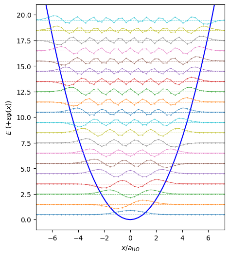
Here we numerically check these methods, first with a 1D harmonic oscillator, which has a simple analytic solution \(E_n = \hbar \omega (n+\tfrac{1}{2})\) and no singularities, then with the Coulomb potential.

In this code, we build these tri-diagonal matrices simply using numpy.diag(), then solve them using the generalized eigenvalue solve scipy.linalg.eig().

import scipy.linalg
import scipy as sp

# Harmonic oscillator in an optimal box for Fourier methods
# to get 20 states with machine precision.
N = 64
L = 20.0
a = dx = L/N
n = np.arange(N)
x = n*dx - L//2

N_states = 30
hbar = m = w = 1

Vx = m*(w*x)**2/2
En = hbar*w*(np.arange(N) + 0.5)  # Exact solution

D2 = (np.diag(np.ones(N-1), k=1) 
      -2*np.diag(np.ones(N)) 
      + np.diag(np.ones(N-1), k=-1))

I = (np.diag(np.ones(N-1), k=1) 
     + 10*np.diag(np.ones(N)) 
     + np.diag(np.ones(N-1), k=-1))/12

V = np.diag(Vx)

fig, ax = plt.subplots()

# Finite Difference
H = -hbar**2/2/m * D2/a**2 + V
E, psi = sp.linalg.eig(H)
inds = np.argsort(abs(E))
E, psi = E[inds], psi[:, inds]
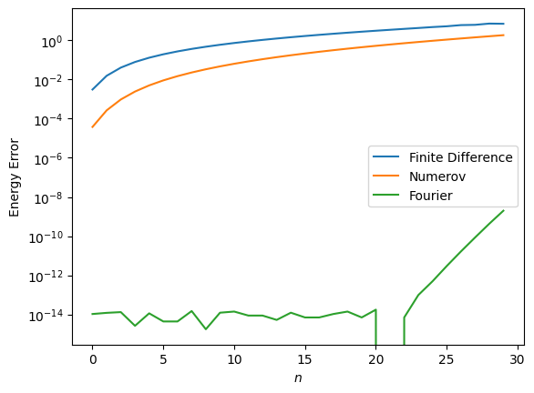
ax.semilogy(n[:N_states], abs(E-En)[:N_states], label="Finite Difference")

# Numerov
H = -hbar**2/2/m * D2/a**2 + I@V
E, psi = sp.linalg.eig(H, I)
inds = np.argsort(abs(E))
E, psi = E[inds], psi[:, inds]
ax.semilogy(n[:N_states], abs(E-En)[:N_states], label="Numerov")

# Fourier

# Here is how to compute K by applying the FFT to he identity
k = 2*np.pi * np.fft.fftfreq(N, a)
K = np.fft.ifft(hbar**2*k**2/2/m * np.fft.fft(np.eye(N), axis=1), axis=1)

# Here is the formula from the notes to check.
U = np.exp(2j*np.pi * n[:, None]*n[None, :]/N)/np.sqrt(N)
n_ = (n + N//2) % N - N//2
k = (2*np.pi * n_/ L)
K = U @ np.diag((hbar*k)**2/2/m) @ U.T.conj()

H = K + V
E, psi = sp.linalg.eigh(H)
#inds = np.argsort(abs(E))
#E, psi = E[inds], psi[:, inds]
ax.semilogy(n[:N_states], abs(E-En)[:N_states], label="Fourier")

ax.set(xlabel="$n$", ylabel="Energy Error")
ax.legend();

This looks promising, but to really check out code, we should make sure we have the appropriate scaling:

hbar = m = w = 1
L = 20.0
N_states = 20
En = hbar*w*(np.arange(N_states) + 0.5)  # Exact solution

Ns = N_states * 2**np.arange(1, 6)
errs = dict(FD=[], Numerov=[])
for N in Ns:
    a = dx = L/N
    n = np.arange(N)
    x = n*dx - L//2
    V = np.diag(m*(w*x)**2/2)
    D2 = (np.diag(np.ones(N-1), k=1) - 2*np.diag(np.ones(N)) + np.diag(np.ones(N-1), k=-1))
    K = -hbar**2/2/m * D2/a**2
    I = (np.diag(np.ones(N-1), k=1) + 10*np.diag(np.ones(N)) + np.diag(np.ones(N-1), k=-1))/12
    
    # Finite Differences
    E = sp.linalg.eigvalsh(K+V)
    errs['FD'].append(abs(E[:N_states]/En - 1))
    
    # Numerov
    H = -hbar**2/2/m * D2/a**2 + I@V
    E = sp.linalg.eigvals(K+I@V, I)
    inds = np.argsort(abs(E))
    E = E[inds]
    errs['Numerov'].append(abs(E[:N_states]/En - 1))

fig, ax = plt.subplots()

as_ = L/Ns
ax.loglog(as_, errs['FD'], ':o')
ax.loglog(as_, errs['Numerov'], '--+')
ax.plot(as_, as_**2, ':k', lw=4, alpha=0.5, label="$a^2$ (Finite Difference)")
ax.plot(as_, as_**4, '--k', lw=4, alpha=0.5, label="$a^4$ (Numerov)")
ax.set(xlabel="$a=L/N$", ylabel="Relative Energy Error")
ax.legend();

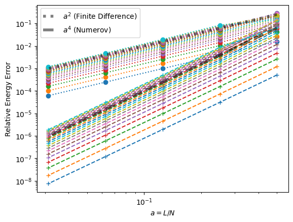
This test confirms that we have correctly implemented the two methods.

Here we will consider only the spherically symmetric (\(S\)-wave) orbits and phase-shifts \(l=m=0\) with constant spherical harmonics \(Y_{0}^{0}(\theta, \phi)\). If you are not familiar with these, you should consider them as “Fourier” components on the sphere. This is most obvious for \(l=0\) where \(Y_{0}^{m}(\theta, \phi) \propto e^{\I m\phi}\) are plane waves. The \(\theta\) dependence is more complicated due to the coordinate system.

Hydrogen Atom

For testing we use the exact energies for the non-relativistic hydrogen atom:

\[\begin{gather*} V(r) = \frac{-\alpha}{r}, \qquad E_{l,n} = \frac{-m\alpha^2/\hbar^2}{2(1+l+n)^2}. \end{gather*}\]

The eigenstates can also be expressed analytically:

\[\begin{gather*} \psi_{n,l,m}(r, \theta, \phi) \propto e^{r/na}\left(\frac{2r}{na}\right)^{l} L_{n-l-1}^{2l+1}\left(\frac{2r}{na}\right)Y_{l}^{m}(\theta, \phi), \qquad a = \frac{\hbar^2}{m \alpha}, \end{gather*}\]

where \(m\) is the reduced mass \(m = m_em_p/(m_e+m_p)\), \(a\) is the reduced Bohr radius, \(L_{n-l-1}^{2l+1}(\rho)\) is a generalized Laguerre polynomial of degree \(n-l-1\), and \(Y_{l}^{m}(\theta, \phi)\) is a spherical harmonic function of degree \(l\) and order \(m\).

These exact solutions might be used to deal with the singular properties of the Coulomb potential, but we postpone discussing this for now in favour of more general techniques.

import scipy.linalg
import scipy as sp

# Hydrogen atom
N = 64*8
R = 20.0
a = R/N
n = np.arange(N)
r = (n + 1)*a

N_states = 30
hbar = m = alpha = 1

Vr = -alpha/r
l = 0
En = -m*alpha**2/hbar**2/2/(1+l+n)**2

D2 = (np.diag(np.ones(N-1), k=1) 
      -2*np.diag(np.ones(N)) 
      + np.diag(np.ones(N-1), k=-1))

I = (np.diag(np.ones(N-1), k=1) 
     + 10*np.diag(np.ones(N)) 
     + np.diag(np.ones(N-1), k=-1))/12

V = np.diag(Vr)

fig, axs = plt.subplots(2, 1)

ax = axs[0]

# Finite Difference
H = -hbar**2/2/m * D2/a**2 + V
E, psi = sp.linalg.eig(H)
inds = np.argsort(E.real)
E, psi = E[inds], psi[:, inds]
ax.semilogy(n[:N_states], abs(E/En-1)[:N_states], label="Finite Difference")
print(En[:4])
print(E[:4].real)

axs[1].plot(r, abs(psi[:,0])**2)
axs[1].plot(r, abs(psi[:,1])**2)

# Numerov
H = -hbar**2/2/m * D2/a**2 + I @ V
E, psi = sp.linalg.eig(H, I)
inds = np.argsort(E.real)
E, psi = E[inds], psi[:, inds]
axs[1].plot(r, abs(psi[:,0])**2)
axs[1].plot(r, abs(psi[:,1])**2)
ax.semilogy(n[:N_states], abs(E/En-1)[:N_states], label="Numerov");
print(E[:4].real)

[-0.5        -0.125      -0.05555556 -0.03125   ]
[-0.49980941 -0.12497557 -0.04998816  0.01634702]

[-0.4995119  -0.1249264  -0.04996446  0.01638553]

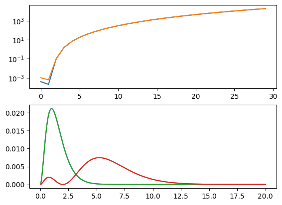
We now see that, although we qualitatively correct solutions, we only have 3 bound states (because our box gets too small), and about 4 places of accuracy, even with a lot of points.

For high accuracy, we probably need to shoot, or be clever.

See Also

• Physics 555: Bound States in the 1D Schrödinger Equation