Show code cell content Hide code cell content

import mmf_setup;mmf_setup.nbinit()
import logging;logging.getLogger('matplotlib').setLevel(logging.CRITICAL)
%matplotlib inline
import numpy as np, matplotlib.pyplot as plt

$\newcommand{\vect}[1]{\mathbf{#1}} \newcommand{\uvect}[1]{\hat{#1}} \newcommand{\abs}[1]{\lvert#1\rvert} \newcommand{\norm}[1]{\lVert#1\rVert} \newcommand{\I}{\mathrm{i}} \newcommand{\ket}[1]{\left|#1\right\rangle} \newcommand{\bra}[1]{\left\langle#1\right|} \newcommand{\braket}[1]{\langle#1\rangle} \newcommand{\Braket}[1]{\left\langle#1\right\rangle} \newcommand{\op}[1]{\mathbf{#1}} \newcommand{\mat}[1]{\mathbf{#1}} \newcommand{\d}{\mathrm{d}} \newcommand{\D}[1]{\mathcal{D}[#1]\;} \newcommand{\pdiff}[3][]{\frac{\partial^{#1} #2}{\partial {#3}^{#1}}} \newcommand{\diff}[3][]{\frac{\d^{#1} #2}{\d {#3}^{#1}}} \newcommand{\ddiff}[3][]{\frac{\delta^{#1} #2}{\delta {#3}^{#1}}} \newcommand{\floor}[1]{\left\lfloor#1\right\rfloor} \newcommand{\ceil}[1]{\left\lceil#1\right\rceil} % The following allows KaTeX to render these for significantly improved % performance on CoCalc. \newcommand{\DeclareMathOperator}[2]{\newcommand{#1}{#2}} \DeclareMathOperator{\Tr}{Tr} \DeclareMathOperator{\erf}{erf} \DeclareMathOperator{\erfi}{erfi} \DeclareMathOperator{\sech}{sech} \DeclareMathOperator{\sn}{sn} \DeclareMathOperator{\cn}{cn} \DeclareMathOperator{\dn}{dn} \DeclareMathOperator{\sgn}{sgn} \DeclareMathOperator{\order}{O} \DeclareMathOperator{\diag}{diag} % \newcommand{\mylabel}[1]{\label{#1}\tag{#1}} \newcommand{\degree}{\circ}$

This cell adds /home/docs/checkouts/readthedocs.org/user_builds/physics-581-the-standard-model/checkouts/latest/src to your path, and contains some definitions for equations and some CSS for styling the notebook. If things look a bit strange, please try the following:

• Choose "Trust Notebook" from the "File" menu.
• Re-execute this cell.
• Reload the notebook.

Mock QFT

Zee’s “baby” problem is the 1D case with \(A = m^2/2\).

To help simplify notations a little later, we express the first part of the exponent as the “Lagrangian”

\[\begin{gather*} L(\vect{q}, \lambda) = \frac{\vect{q}^T\mat{A}\vect{q}}{2} + \frac{\lambda}{4!}q^4. \end{gather*}\]

Then we can define the following probability distribution over \(\vect{q}\):

\[\begin{gather*} \rho(\vect{q}, \lambda) = \frac{e^{-L(\vect{q},\lambda)}} {Z(\vect{0}, \lambda)}. \end{gather*}\]

We will use this notion later.

We start with Zee’s “child” problem [Zee, 2010] which asks us to consider the following integral

\[\begin{gather*} Z(\vect{J}, \lambda) = \int\d^{N}\vect{q}\; \exp\Biggl( \overbrace{ -\frac{\vect{q}^T\mat{A}\vect{q}}{2} - \frac{\lambda}{4!}q^4}^{-L(\vect{q}, \lambda)} + \vect{J}\vect{q} \Biggr), \qquad q^4 = \sum_{i}q_i^4. \end{gather*}\]

Performing the gaussian integrals, we get

\[\begin{gather*} Z(\vect{J}, \lambda) = \underbrace{ \overbrace{\sqrt{\frac{(2\pi)^N}{\det\mat{A}}}} ^{\frac{1}{\sqrt{\det(\mat{A}/2\pi)}}}}_{Z(0,0)} \exp\left(-\frac{\lambda}{4!}\sum_{i}\diff[4]{}{J_i}\right) \exp\left(\frac{1}{2}\vect{J}^T\mat{A}^{-1}\vect{J}\right). \end{gather*}\]

We can express this as a power series in \(\vect{J}\),

\[\begin{gather*} \frac{Z(J, \lambda)}{Z(0,0)} = \sum_{s=0}^{\infty} \frac{1}{s!}G^{(s)}_{i_1i_2\dots i_s}J_{i_1}J_{i_2}\cdots J_{i_s} \end{gather*}\]

where the indices \(i_n\) are implicitly summed over. From this it might be clear that the \(G^{(s)}_{\vect{i}}(\lambda)\) behave like moments over the distribution \(\rho(\vect{q}, \lambda)\) defined in the margin note above:

\[\begin{align*} G^{(s)}_{i_1i_2\dots i_s}(\lambda) &= \left. \frac{1}{Z(\vect{0},0)} \frac{\partial^s Z(\vect{J}, \lambda)} {\partial J_{i_1}\partial J_{i_2} \dots \partial J_{i_s}}\right|_{\vect{J} = 0} \\ &= \frac{1}{Z(0,0)} \int \d^{N}\; q_{i_1}q_{i_2}\dots q_{i_s} \exp\left( -\frac{\vect{q}^T\mat{A}\vect{q}}{2} -\frac{\lambda}{4!}q^4 \right)\\ &= \frac{Z(\vect{0},\lambda)}{Z(\vect{0},0)} \braket{q_{i_1}q_{i_2}\cdots q_{i_s}}_{e^{-L(\vect{q}, \lambda)}}. \end{align*}\]

The source term \(\vect{J}\) is simply a tool for computing these moments.

Analogy with Field Theory

Think of the indices \(i_n\) as specifying a location: i.e. a site on a 1D lattice \(x_n = ai_n\) where \(a\) is the lattice spacing. The quantity \(G^{(s)}_{i_1 i_2 \dots i_s}(\lambda)\) are analogous to the \(s\)-point Green’s functions, which are primary quantities of interest in quantum field theory. For example, the 2-point function \(G^{(2)}_{ij}\) plays the role of the propagator, describing how a particle “propagates” from site \(i\) to site \(j\).

The goal of perturbative field theory is to calculate quantities like the full propagator \(G^{(2)}_{ij}(\lambda)\) using a perturbation theory based on Feynman diagrams whose ingredients are quantities like the bare propagator \(G^{(2)}_{ij}(0)\). Note that the bare propagator has a simple form:

\[\begin{gather*} G^{(2)}_{ij}(\lambda = 0) = [\mat{A}^{-1}]_{ij} \end{gather*}\]

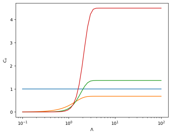
Here we expand Zee’s “baby problem” [Zee, 2010] to include ideas about renormalization. To this end, imagine that we can perform “experiments” which “measure” the value of \(N\)-point “correlation functions” at some \(\Lambda\):

\[\begin{gather*} \newcommand{\Z}{\mathcal{Z}} C_n(\Lambda) = \frac{1}{\Z(0, \Lambda)}\left.\diff[n]{}{J}\Z(J, \Lambda)\right|_{J=0}, \qquad \Z(J, \Lambda) = \Z(0, \Lambda)\sum_{n=0}^{\infty} C_n(\Lambda) \frac{J^n}{n!}. \end{gather*}\]

To be consistent with Zee’s problem, we assume that we have a symmetry \(J \rightarrow -J\) so that only even terms are non-zero. To be definite, let

\[\begin{gather*} \Z(J, \Lambda) = \int_{-\Lambda}^{\Lambda}\d{q}\; e^{-L(q) + Jq}, \qquad L(q) = \frac{m^2}{2}q^2 + \frac{\lambda}{4!}q^4, \end{gather*}\]

where the parameters \(m\) and \(\lambda\) are “fundamental parameters of nature”. We will compute the results of these “measurements” numerically by simply doing the integral once we have chosen the parameters:

These measurements are just the various “moments” of the probability distribution \(\rho(q) \propto e^{-L(q)}\) normalized on the interval \([-\Lambda, \Lambda]\).

\[\begin{gather*} C_n(\Lambda) = \braket{q^n} = \frac{\int_{-\Lambda}^{\Lambda}\d{q}\; q^n e^{-L(q)}} {\int_{-\Lambda}^{\Lambda}\d{q}\; e^{-L(q)}}. \end{gather*}\]

We would like to model this using the following theory – our “mock QFT”

\[\begin{gather*} Z(J, \Lambda) = \int_{-\infty}^{\infty}\d{q}\; e^{-L_{\Lambda}(q)+ Jq}, \\ L_{\Lambda}(q) = c_0(\Lambda) + c_2(\Lambda)q^2 + c_4(\Lambda)q^4 + c_6(\Lambda) q^6 + \cdots. \end{gather*}\]

In the limit \(\Lambda \rightarrow \infty\), our theory should “agree with nature”, with \(c_0(\infty) = 0\), \(c_2(\infty) = m^2/2\), and \(c_4(\infty) = \lambda/4!\), but at finite scales \(\Lambda\), we may need additional coefficients that depend on the scale \(c_n(\Lambda)\). In our “theory”, we have moved the scale dependence \(\Lambda\) into the coefficients \(c_n(\Lambda)\) so that we can complete the gaussian integral as with Zee’s baby problem. The technique for calculating the various “correlation functions” \(C_n(\Lambda)\) is the same in terms of “Feynman” diagrams, but now possibly with more interactions.

from functools import partial
from scipy.integrate import quad
m = 1.2
lam = 0.1
def integrand(q, n):
    return q**n * np.exp(-m**2/2*q**2-lam/4/3/2*q**4)
    
def get_C(n, Lam):
    kw = dict(epsabs=1e-12, epsrel=1e-12)
    Zn = quad(partial(integrand, n=n), -Lam, Lam, **kw)[0]
    Z0 = quad(partial(integrand, n=0), -Lam, Lam, **kw)[0]
    return Zn/Z0

Lams = 10**np.linspace(-1, 2)
ns = [0, 2, 4, 6]
Cs = np.array([[get_C(n, Lam) for Lam in Lams] for n in ns])
fig, ax = plt.subplots()
ax.semilogx(Lams, Cs.T)
ax.set(xlabel=r"$\Lambda$", ylabel="$C_n$");