Show code cell content Hide code cell content

import mmf_setup;mmf_setup.nbinit()
import logging;logging.getLogger('matplotlib').setLevel(logging.CRITICAL)
%matplotlib inline
import numpy as np, matplotlib.pyplot as plt

$\newcommand{\vect}[1]{\mathbf{#1}} \newcommand{\uvect}[1]{\hat{#1}} \newcommand{\abs}[1]{\lvert#1\rvert} \newcommand{\norm}[1]{\lVert#1\rVert} \newcommand{\I}{\mathrm{i}} \newcommand{\ket}[1]{\left|#1\right\rangle} \newcommand{\bra}[1]{\left\langle#1\right|} \newcommand{\braket}[1]{\langle#1\rangle} \newcommand{\Braket}[1]{\left\langle#1\right\rangle} \newcommand{\op}[1]{\mathbf{#1}} \newcommand{\mat}[1]{\mathbf{#1}} \newcommand{\d}{\mathrm{d}} \newcommand{\D}[1]{\mathcal{D}[#1]\;} \newcommand{\pdiff}[3][]{\frac{\partial^{#1} #2}{\partial {#3}^{#1}}} \newcommand{\diff}[3][]{\frac{\d^{#1} #2}{\d {#3}^{#1}}} \newcommand{\ddiff}[3][]{\frac{\delta^{#1} #2}{\delta {#3}^{#1}}} \newcommand{\floor}[1]{\left\lfloor#1\right\rfloor} \newcommand{\ceil}[1]{\left\lceil#1\right\rceil} % The following allows KaTeX to render these for significantly improved % performance on CoCalc. \newcommand{\DeclareMathOperator}[2]{\newcommand{#1}{#2}} \DeclareMathOperator{\Tr}{Tr} \DeclareMathOperator{\erf}{erf} \DeclareMathOperator{\erfi}{erfi} \DeclareMathOperator{\sech}{sech} \DeclareMathOperator{\sn}{sn} \DeclareMathOperator{\cn}{cn} \DeclareMathOperator{\dn}{dn} \DeclareMathOperator{\sgn}{sgn} \DeclareMathOperator{\order}{O} \DeclareMathOperator{\diag}{diag} % \newcommand{\mylabel}[1]{\label{#1}\tag{#1}} \newcommand{\degree}{\circ}$

This cell adds /home/docs/checkouts/readthedocs.org/user_builds/physics-581-the-standard-model/checkouts/latest/src to your path, and contains some definitions for equations and some CSS for styling the notebook. If things look a bit strange, please try the following:

• Choose "Trust Notebook" from the "File" menu.
• Re-execute this cell.
• Reload the notebook.

Scalar Field Theory

Here we work through some details of the scalar field theory of phonons developed in [Donoghue and Sorbo, 2022]. Equation number references are to this textbook.

Path Integral

We start with the path integral (8.37) as a generating functional:

A couple of notes. We generalize to \(d\) dimensions, and allow for arbitrary interaction terms \(c_n\phi^{n}/4!\) with coefficients \(c_n\) where \(c_2 = m^2\) and \(c_4 = \lambda\). This will enable more general discussions of RG flow later. We also use the more customary notation of \(\mathcal{D}[\phi]\) for the measure of the path integral.

\[\begin{gather*} Z_{\vect{c}}[J] = N\int\mathcal{D}[\phi]e^{-S_{\vect{c}}[\phi]/\I\hbar}, \qquad S_{\vect{c}}[\phi] = \int \d^{d}{x}\; \Bigl(\mathcal{L}_{\vect{c}}(\phi) + J(x)\phi(x)\Bigr)\\ \mathcal{L}_{\vect{c}}(\phi) = \frac{1}{2}\partial_{\mu}\phi\partial^{\mu}\phi \underbrace{\;- \frac{m^2}{2}\phi^2(x) - \frac{\lambda}{4!}\phi^4(x)} _{-\sum_{n}\frac{c_n}{n!}\phi^n(x)}. \end{gather*}\]

Perturbative Expansion

To work with this perturbatively, we separate the quadratic piece from the rest, which we call the interactions:

\[\begin{gather*} \mathcal{L}_{\vect{c}}(\phi) = \underbrace{\frac{1}{2}\partial_{\mu}\phi\partial^{\mu}\phi - \frac{m^2}{2}\phi^2(x)} _{\mathcal{L}_{0}} \underbrace{-\sum_{n>2}\frac{c_n}{n!}\phi^n(x)}_{\mathcal{L}_{I}}. \end{gather*}\]

The idea here is that we know how to explicitly solve for the quadratic terms by completing the square (8.21):

\[\begin{gather*} Z_0[J] = N \int\mathcal{D}[\phi]e^{-\int\d^d{x}\bigl( \mathcal{L}_0(\phi) + J(x)\phi(x)\bigr)/\I\hbar}. \end{gather*}\]

To compute the additional terms, we simply differentiate (8.38):

\[\begin{gather*} Z_{\vect{c}}[J] = e^{\int \d^d{x}\mathcal{L}_{I}\bigl(-\I\delta/\delta J(x)\bigr)}Z_0[J]. \end{gather*}\]

Expanding this first exponential in powers of the coupling constants \(c_n\) gives the perturbative expansion.

Propagator

To proceed, we must compute the quadratic path integral (8.21). This can be done by completing the square, and introducing a convergence factor (8.22) resulting in the expression (8.28)

\[\begin{gather*} Z_0[J] = Z_0[0]\exp\left\{ -\frac{1}{2}\int\d^d{x}\d^d{y}\;J(x)\I \hbar D_F(x-y)J(y) \right\}. \end{gather*}\]

This should be compared with the child problem §I.7(9) in [Zee, 2010]:

\[\begin{gather*} Z(\vect{J}) = \underbrace{\sqrt{\frac{(2\pi)^{N}}{\det[\mat{A}]}}}_{Z_0(0)} e^{-(\lambda/4!)\sum_{i}(\partial/\partial J_i)^4} e^{\frac{1}{2}\vect{J}\cdot\mat{A}^{-1}\vect{J}}. \end{gather*}\]

From this, we see that the propagator \(-\I \hbar D_F(x-y)\) can be thought of as the matrix elements \([\mat{A}^{-1}]_{xy}\) taken to the continuum limit where the matrix indices are the space-time coordinates \(x\) and \(y\).

Following this analogy, we have that \(-S_0(\phi)/\I\hbar \equiv -\tfrac{1}{2}\vect{q}\cdot\mat{A}\cdot \vect{q}\) where \(\phi(x) \equiv [\vect{q}]_{x}\):

\[\begin{gather*} \frac{S_0(\phi)}{\I\hbar} = \frac{1}{2\I\hbar} \int \d^d{x}\bigl( \partial_{\mu}\phi\partial^{\mu}\phi - m^2\phi^2(x) \bigr)\\ = \frac{1}{2}\int \d^d{x}\d^d{y}\;\phi(x) \underbrace{ \frac{\delta^{d}(x-y)\bigl[-\partial_{\mu}\partial^{\mu} - m^2\bigr]}{\I\hbar} }_{[-\mat{A}]_{xy}}\phi(y), \end{gather*}\]

we see that \(\mat{A}\mat{A}^{-1} = \mat{1}\) is equivalent (after integrating the first term by parts) to

\[\begin{gather*} \int\d^{d}{y}\; \underbrace{ \frac{\delta^{d}(x-y)\bigl[-\partial_{\mu}\partial^{\mu} - m^2\bigr]}{-\I\hbar} }_{[\mat{A}]_{xy}} \underbrace{\frac{\hbar D_F(y-z)}{\I}}_{[\mat{A}^{-1}]_{yz}} = \underbrace{\delta^{d}(x-z)}_{[\mat{1}]_{xz}}. \end{gather*}\]

In other words, the propagator \(D_F(x-y)\) is a Green’s function (8.24):

\[\begin{gather*} \bigl(\partial_\mu\partial^\mu + m^2\bigr)D_F(x) = -\delta^{d}(x). \end{gather*}\]

Causality and Convergence

Here we face an issue: the operator \(\partial_\mu\partial^\mu + m^2\) is singular (has zero eigenfunctions), meaning that \(\mat{A}\) cannot be inverted, and therefore that there is not a unique solution for \(D_F(x)\). To resolve this, one typically adds a convergence factor, in the book written as \(\I\epsilon\) in (8.24):

\[\begin{gather*} \bigl(\partial_\mu\partial^\mu + m^2 - \I\epsilon\bigr)D_F(x) = -\delta^{d}(x). \end{gather*}\]

This resolves the singularities and uniquely defines what is known as the Feynman propagator (hence the subscript \(F\)). Several other options are common.

To elucidate the meaning, we first consider a field theory in \(d=1\) dimension (no space):

\[\begin{gather*} \left(-\diff[2]{}{t} - m^2\right)D(t) = \delta(t). \end{gather*}\]

This is an inhomogeneous linear differential equation. The general homogeneous solution is

\[\begin{gather*} a_{+}e^{\I\omega t} + a_{-}e^{-\I\omega}, \qquad \omega = \tfrac{c^2}{\hbar}m. \end{gather*}\]

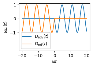
The inhomogeneous solution can be found by stitching together these solutions such that the function is continuous, but the derivative has a unit step at \(t=0\):

Recall that the derivative of the unit (Heaviside) step function is a Dirac delta function:

\[\begin{gather*} \Theta'(t) = \delta(t). \end{gather*}\]

\[\begin{gather*} D(t) = \begin{cases} a_{+}e^{\I\omega t} + a_{-}e^{-\I\omega} & t < 0,\\ b_{+}e^{\I\omega t} + b_{-}e^{-\I\omega} & t > 0. \end{cases},\\ \qquad D(+\epsilon) = D(-\epsilon), \qquad D'(+\epsilon) - D'(-\epsilon) = -1, \\ a_{+} + a_{-} = b_{+} + b_{-}, \qquad b_{+} - b_{-} = \frac{\I}{\omega} + a_{+} - a_{-},\\ D(t) = \begin{cases} a_{+}e^{\I\omega t} + a_{-}e^{-\I\omega} & t < 0,\\ a_{+}e^{\I\omega t} + a_{-}e^{-\I\omega} - \frac{1}{\omega}\sin \omega t & t > 0. \end{cases}. \end{gather*}\]

Fig. 3 Advanced and retarded propagators (Green’s functions) for a 1-dimensional field theory (no space) with mass \(m = \tfrac{\hbar}{c^2} \omega\).

We have expressed this general solution as the general homogeneous solution plus the advanced Green’s function \(D_{\mathrm{adv}}(t)\) which vanishes for \(t<0\). One can also define the retarded or causal \(D_{\mathrm{ret}}(t)\) Green’s function, which vanishes for \(t>0\) c.f. (4.47).

\[\begin{gather*} D_{\mathrm{adv}}(t) = -\Theta(t)\frac{\sin\omega t}{\omega}, \qquad D_{\mathrm{ret}}(t) = \Theta(-t)\frac{\sin\omega t}{\omega}. \end{gather*}\]

Show code cell content Hide code cell content

from myst_nb import glue

w = 10
t = np.linspace(-20, 20, 200)/w
fig, ax = plt.subplots(figsize=(3, 2))
D_adv = np.where(t>0, -np.sin(w*t)/w, 0)
D_ret = np.where(t<0, np.sin(w*t)/w, 0)
ax.plot(w*t, w*D_adv, label=r"$D_{\mathrm{adv}}(t)$")
ax.plot(w*t, w*D_ret, label=r"$D_{\mathrm{ret}}(t)$")
ax.set(ylim=(-2.3, 1.1), yticks=[-1, 0, 1], 
       xlabel=r"$\omega t$", ylabel=r"$\omega D(t)$")
ax.legend()
glue("fig_propagators", fig, display=False);

Do It! Use the Green’s function to do some sourcery.

Use the Green’s function to solve the Klein-Gordon equation for an external source that is a step function:

\[\begin{gather*} J(t) = J_0\begin{cases} 1 & 0 < t < t_0\\ 0 & \text{otherwise}. \end{cases} \end{gather*}\]

I.e. start with the vacuum state at early times \(t \rightarrow -\infty\) and solve the Klein-Gordon equation with this source:

\[\begin{gather*} \left(\diff[2]{}{t} + m^2\right)\phi(t) = J(t). \end{gather*}\]

Hint: Express \(J(t)\) as a “sum” of delta-functions, then write the solution as the same “sum” using \(D_{\mathrm{adv}}(t)\).

Solution

The standard use of Green’s functions is:

\[\begin{gather*} J(t) = \int\d{t'} \delta(t-t')J(t')\\ \underbrace{\left(\diff[2]{}{t} + m^2\right)}_{\op{O}_{KG}}\phi_J(t) = \int\d{t'} \delta(t-t')J(t')\\ \phi_J(t) = -\int D(t-t')J(t')\d{t'}\\ \end{gather*}\]

(C.f. (4.48).) Proof:

\[\begin{gather*} \op{O}_{KG}\phi_J(t) = \int \op{O}_{KG}D(t-t')J(t')\d{t'} = \int -\delta(t-t')J(t')\d{t'} = J(t). \end{gather*}\]

Explicit form: \(u=t-t'\), \(\d{u} = -\d{t'}\)

\[\begin{align*} \phi_J(t) &= J_0 \int_{0}^{t_0}\frac{\Theta(t-t')\sin\bigl(\omega (t-t')\bigr)}{\omega}\d{t'},\\ &= -J_0 \int_{t}^{t-t_0}\frac{\Theta(u)\sin\bigl(\omega u\bigr)}{\omega}\d{u},\\ &= -J_0 \int_{\max(t,0)}^{\max(t-t_0, 0)}\frac{\sin\omega t'}{\omega} \d{t'},\\ &= J_0 \cos\omega t'\Big|^{\max(t-t_0, 0)}_{\max(t, 0)} \end{align*}\]

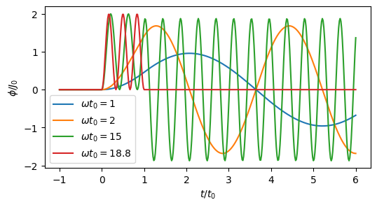
Fig. 4 Here are some solutions.

Show code cell content Hide code cell content

t0 = 1
fig, ax = plt.subplots(figsize=(6, 3))
t = np.linspace(-1, 6, 400)*t0
J0 = 1
for w in [1, 2, 15, 6*np.pi]:
    phi = J0*(np.cos(w*np.maximum(t-t0, 0)) - np.cos(w*np.maximum(t, 0)))
    ax.plot(t/t0, phi/J0, label=f"$\omega t_0={w*t0:.3g}$")
ax.set(xlabel=r"$t/t_0$", ylabel=r"$\phi/J_0$")
ax.legend();
glue("fig_step_solution", fig, display=False);

The convention for the Fourier transform here gives the usual signs for the spatial components, and a negative sign for the time:

\[\begin{gather*} e^{-\I p_\mu x^{\mu}} = e^{-\I (p^0x^0 - \vect{p}\cdot\vect{x})}\\ = e^{-\I \omega t + \I \vect{p}\cdot\vect{x}}. \end{gather*}\]

With this convention, the \(\partial_{\mu} \rightarrow = -\I p_\mu\), hence the change of sign \(\partial_\mu \partial^\mu \rightarrow -p^2\).

Although this was easily solved, let’s also directly evaluate this using Fourier techniques, which will generalize to higher dimension.

\[\begin{gather*} D(x) = \int \frac{\d^d{p}}{(2\pi)^d}\;e^{-\I p_\mu x^\mu}\tilde{D}(p), \qquad \delta^{d}(x) = \int \frac{\d^d{p}}{(2\pi)^d}\;e^{-\I p_\mu x^\mu},\\ (p^2 - m^2)\tilde{D}(p) = (p_0^2 - \vect{p}^2 - m^2) \tilde{D}(p) = 1. \end{gather*}\]

Thus, formally,

\[\begin{gather*} \tilde{D}(p) = \frac{1}{p^2 - m^2}, \end{gather*}\]

though, again, this is singular and thus not well defined until we include a convergence factor. As is done in [Donoghue and Sorbo, 2022] (8.24), one commonly sees this added as

\[\begin{gather*} \tilde{D}_F(p) = \frac{1}{p^2 - m^2 + \I \epsilon}. \end{gather*}\]

Note

I prefer to do this slightly differently by promoting \(E \equiv p_0 \rightarrow (1+\I 0^+)p_0\) where I use the notation \(0^+ \equiv \epsilon\) to be explicit about the sign. In this propagator, these are equivalent:

\[\begin{gather*} \frac{1}{p_0^2(1+\I 0^+)^2 - \vect{p}^2 - m^2} = \frac{1}{p_0^2+ \underbrace{2p_0^2\I 0^+}_{\equiv \I \epsilon} - \vect{p}^2 - m^2} \end{gather*}\]

However, in other cases, the correct procedure is to shift the poles based on the sign of the energy, so affixing the convergence factor to \(E\equiv p_0\) is more generally valid.

Fig. 5 Contours.

Contours required to compute the propagator. Note that if \(t>0\), we need to close the contour in the upper half-plane so that the exponent \(e^{\I\omega t}\) vanishes at infinity. This will pickup the negative-energy pole. If \(t<0\), we need to close the contour down in the lower half-plane, picking up the positive energy pole. Integrating counter-clockwise will give a sum of the poles with factors of \(2\pi \I\) times the residue. Closing down changes the sign.

To compute the propagator in real space, we can now perform the integral over \(p_0\) as a contour integral (see Fig. Contours.):

Show code cell content Hide code cell content

from myst_nb import glue

t = np.linspace(-1, 1)
th = np.linspace(0, np.pi)
E = 0.5
ie = 0.1j
ws = np.array([E*(1-ie), -E*(1-ie)])
fig, ax = plt.subplots(figsize=(3, 3))

ax.plot(ws.real, ws.imag, 'xk')
ax.plot(t, 0.2*abs(ie)+0*t, 'C0-')
ax.plot(np.cos(th), np.sin(th), 'C0-', label="$t<0$")
ax.plot(t, -0.2*abs(ie)+0*t, 'C1-')
ax.plot(np.cos(th), -np.sin(th), 'C1-', label="$t>0$")
ax.set(xlabel=r"$\Re\omega$", ylabel=r"$\Im \omega$")
ax.legend()
glue("fig_contour", fig, display=False);

\[\begin{gather*} \tilde{D}_F(t, \vect{p}) = \int_{-\infty}^{\infty} \frac{\d{p_0}}{2\pi} \frac{e^{\overbrace{-\I p_0 x^0}^{-\I \omega t}}}{p_0^2 - \vect{p}^2 - m^2 + \I 0^+} = \oint\frac{\d{\omega}}{2\pi} \frac{e^{-\I\omega t}}{[\omega(1+\I 0^+)]^2 - \vect{p}^2 - m^2}. \end{gather*}\]

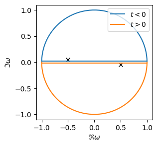
To do this integral, note that the integrand is an analytic function with two poles:

\[\begin{gather*} \omega = \omega_{\pm}(1-\I 0^+), \qquad \omega_{\pm} = \pm \sqrt{\vect{p^2} + m^2} = \pm E(\vect{p}). \end{gather*}\]

Thus, if the poles are at positive energy, then they are shifted down into the lower half-plane, but if they are negative, then they are shifted up. If \(t>0\), we can close the contour down, picking up the positive-energy pole, otherwise we must close the contour up:

\[\begin{gather*} \tilde{D}_F(t, \vect{p}) \equiv \oint\frac{\d{\omega}}{2\pi} \frac{e^{-\I\omega t}}{\bigl(\omega - \omega_+(1-\I 0^+)\bigr) \bigl(\omega - \omega_-(1-\I 0^+)\bigr)} = \frac{-\I e^{-\I \abs{t} E(\vect{p})}}{2E(\vect{p})}\\ = -\I\frac{\Theta(t)e^{-\I t E(\vect{p})} + \Theta(-t)e^{\I t E(\vect{p})}} {2E(\vect{p})}. \end{gather*}\]

Show code cell content Hide code cell content

# Check that our formula are correct
from scipy.integrate import quad
E = 2.0
e = 0.001

def quadc(f, *v, **kw):
    ri, re = quad(lambda *v: f(*v).real, *v, **kw)
    ii, ie = quad(lambda *v: f(*v).imag, *v, **kw)
    return ri + 1j*ii, re + 1j*ie

def f_F(w, e=e):
    global t
    return np.exp(1j*w*t)/((w*(1+1j*e))**2 - E**2)/2/np.pi
    
def f_ret(w, e=e):
    global t
    return np.exp(1j*w*t)/((w + 1j*e)**2 - E**2)/2/np.pi
    
def f_adv(w, e=e):
    global t
    return np.exp(1j*w*t)/((w - 1j*e)**2 - E**2)/2/np.pi

T = 50
for t in [-1.2, 1.2]:
    D_F = -1j*np.exp(-1j*abs(t)*E)/2/E
    D_adv = -(t>0)*np.sin(E*t)/E
    D_ret = (t<0)*np.sin(E*t)/E, 
    assert np.allclose(quadc(f_F, -T, T)[0], D_F, atol=0.001)
    assert np.allclose(quadc(f_ret, -T, T)[0], D_ret, atol=0.001)
    assert np.allclose(quadc(f_adv, -T, T)[0], D_adv, atol=0.001)
    assert np.allclose(D_F - (D_adv+D_ret)/2, -1j*np.cos(E*t)/2/E)

Do it! Do the contour integral

Performing the contour integral, we obtain:

\[\begin{align*} \tilde{D}_F(t, \vect{p}) &= \begin{cases} \frac{-\I e^{-\I \omega_+ t}}{\omega_+ - \omega_-} & t > 0\\ \frac{\I e^{\I \omega_+ t}}{\omega_- - \omega_+} = \frac{-\I e^{\I \omega_+ t}}{\omega_+ - \omega_-} & t < 0 \end{cases}\\ &= \frac{-\I}{2E(\vect{p})}\begin{cases} e^{-\I t E(\vect{p})} & t > 0\\ e^{\I t E(\vect{p})} & t < 0 \end{cases}\\ &= \frac{-\I e^{-\I \abs{t} E(\vect{p})}}{2E(\vect{p})}. \end{align*}\]

Note

Connecting with our previous discussion of the propagator for the \(d=1\) theory, we note that \(E(\vect{p}) = m\) (which we called \(\omega\) above), so we have

\[\begin{gather*} D_{F}(t) = \frac{-\I e^{-\I \abs{t} m}}{2m} = \frac{-\I \cos(-\abs{t} m) - \sin(-\abs{t} m)}{2m} = \frac{-\I \cos mt + \sin m\abs{t}}{2m}\\ = \frac{-\I \cos m t}{2m} + \frac{\Theta(-t) - \Theta(t)}{2m}\sin mt \\ = \frac{-\I \cos m t}{2m} + \frac{D_{\mathrm{adv}}(t) + D_{\mathrm{ret}}(t)}{2} \end{gather*}\]

Do it! Do I.3.3 from [Zee, 2010].

Show that the advanced and retarded propagators are obtained with \(p_0 \rightarrow p_0 \mp \I 0^+\), or \(\tilde{D}_{\substack{\mathrm{adv}\\\mathrm{rel}}}(p) = 1/(p^2 - m^2 \mp \I \sgn (p_0) 0^{+})\).

Solution

Note that now both poles are shifted in the same direction. Thus, closing the contour either picks up both residues, or picks up neither, depending on the sign of \(t\). This ensures that the propagators are either fully advanced of fully retarded by providing the appropriate \(\Theta(\pm t)\) prefactor. I leave it to you to do the integrals since I have already given the answer above.

To get the real-space propagator, we need to complete the Fourier transform, integrating over the momenta:

\[\begin{gather*} D_F(t, \vect{x}) = \int \d^{d}{p} e^{\I p_{\mu}x^{\mu}}\frac{1}{p^2 - m^2 + \I 0^+} = \int \d^{d-1}{\vect{k}}\; e^{\I\vect{k}\cdot\vect{x}} \frac{-\I e^{\I \abs{t}E(\vect{p})}}{2E(\vect{p})} \end{gather*}\]