Shooting the Radial Schrödinger Equation

Shooting the Radial Schrödinger Equation#

To Do#

Fix asymptotic behaviour at \(r=0\) for \(l>0\).
Improve estimate of \(u_0\) in get_r_u_du_backwards: this is causing major performance issues for large \(n\). If it is set to a reasonable value (so that the maximum solution is order 1) then with a good max_step we get nice convergence.

The simple solution is to use scipy.integrate.solve_ivp() to shoot a solution to some large radius \(R\):

\[\begin{gather*} u(0) = 0, \qquad u'(0) = 1, \qquad u(R)\approx 0. \end{gather*}\]

A couple of issues need to be dealt with:

The integrand is singular at \(r=0\), so we must start from a small non-zero value \(r_0\), thus we replace our boundary conditions with:

\[\begin{gather*} u(r_0) = r_0, \qquad u'(r_0) = 1, \qquad u(R)\approx 0. \end{gather*}\]
The potential extends to \(r\rightarrow \infty\) without falling off very quickly \(V(r) \propto r^{-1}\). Thus, determining what radius \(R\) is “large” is a bit subtle.

Note

The results of this discussion are codified in the phys_581.seq.SEQ class which we use elsewhere. These notes document some of the explorations that led to that code.

from scipy.integrate import solve_ivp
from scipy.interpolate import InterpolatedUnivariateSpline
from scipy.optimize import brentq
from functools import partial

from phys_581 import dvr

d = 3
hbar = m = alpha = 1.0
r0 = 0.2

rng = np.random.default_rng(seed=2)

# 3rd order random polynomial
P = (rng.random(3) - 0.5)*2

def V(r):
    return np.polyval(P, (r/r0)**2) * np.exp(-(r/r0)**2/2) - alpha/np.sqrt(r**2 + r0**2)

def V(r):
    """Hydrogen atom for testing."""
    return -alpha/r

def compute_du_dr(r, u_, E, l=0):
    nu = l + d/2 - 1
    u, du = u_
    ddu = (2*m*(V(r) - E) / hbar**2 + (nu**2-0.25)/r**2)*u
    return (du, ddu)

def get_r_u_du(E, r0=1e-12, R=30.0, R_max=None, tol=1e-8, max_step=0.1, l=0):
    y0 = (r0, 1)
    R_span = (r0, R)
    res = solve_ivp(partial(compute_du_dr, E=E, l=l), t_span=R_span, y0=y0,
                    max_step=max_step, atol=tol, rtol=tol)
    rs = res.t
    us, dus = res.y
    return rs, us, dus

Es = -m*alpha**2/2/hbar**2/ np.arange(1, 20)**2

fig, ax = plt.subplots()
lss = ["-", "--", "-.", ":"]
for _nE, E in enumerate(Es[:3]):
    for _nt, log10_tol in enumerate([-8, -10, -12, -13]):
        r, u, du = get_r_u_du(E=E, tol=10**log10_tol, R=40)
        label = f"tol = $10^{{{log10_tol}}}$" if _nE == 0 else None
        ax.plot(r, u, ls=lss[-1-_nt], c=f"C{_nE}", label=label)
ax.set(ylim=(-1, 1), ylabel='$u(r)$', xlabel="$r$")
ax.legend();

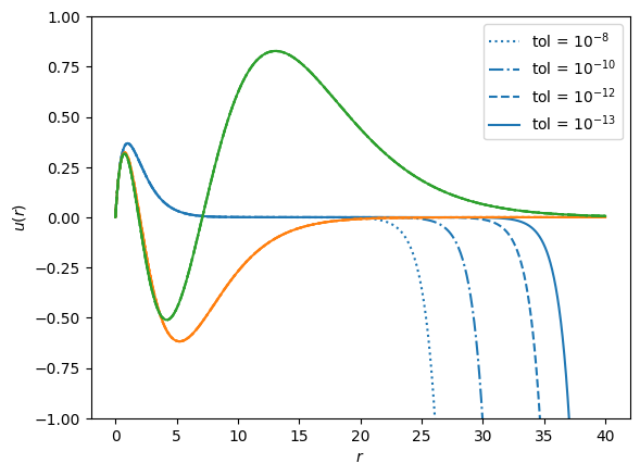
../../_images/2658775a932793c961353611f949497329291f8cda5611255379104dffdd7715.png

We see that this works, but because of the exponentially growing solution for larger \(r\), one needs quite hight tolerances on the integrator. We see another problem, that as the binding energy gets smaller, the radius of the wavefunction gets larger. This will introduce errors in the energy.

These are two different types of errors: the first is a result of the integrator not taking a small enough step size. This is sometimes called an “ultraviolet” (UV) error because it results from short-wavelength physics. The second error is sometimes called an “infrared” (IR) error because it results from long-wavelength physics (our box is not large enough). To get an accurate result, one must understand and mitigate both types of error, each of which increases the computational cost of the calculation.

Let’s complete the simple solution by shooting to find the eigenvalues. We will polish the solution using scipy.optimize.brentq(). This requires a bracket, so we start with a guess for \(E\) then expand our search for a bracket.

import scipy.optimize

def f0(E, **kw):
    """Simple objective function u(R)=0"""
    r, u, du = get_r_u_du(E, **kw)
    return u[-1]

def get_E(E, f=f0, tol=1e-8, lam=0.9, **kw):
    """Shoot for the best E."""
    f_ = partial(f, tol=tol, **kw)
    f0 = f1 = 1
    while f0*f1 > 0:
        lam *= lam
        E0 = lam*E
        E1 = E/lam
        f0, f1 = map(f_, [E0, E1])
    return scipy.optimize.brentq(f_, E0, E1, xtol=tol)

get_E(Es[1], f=f0, R=20)

-0.12498711439290973

We can now explore the errors:

from tqdm import tqdm
from IPython.display import display, clear_output

tols = 10**(np.linspace(-4, -12, 10))
Rs = np.linspace(10.0, 60.0, 10)
R = 30.0
tol = 1e-9

fig, axs = plt.subplots(1, 2, figsize=(10, 5))
ax = axs[0]
for _nE, E in enumerate(Es[:3]):
    Es_ = np.array([get_E(E, R=R, tol=_tol) for _tol in tqdm(tols)])
    ax.loglog(tols, abs(Es_/E - 1), '+-', label=f"$n={_nE}$", c=f"C{_nE}")
ax.axvline([tol], c='y', ls=':')
ax.set(xlabel="tol", ylim=(1e-12, 1e-2), ylabel="rel. error", title="UV Convergence")
ax.legend();

ax = axs[1]
for _nE, E in enumerate(Es[:3]):
    Es_ = np.array([get_E(E, R=_R, tol=tol) for _R in tqdm(Rs)])
    ax.semilogy(Rs, abs(Es_/E - 1), '+-', label=f"$n={_nE}$", c=f"C{_nE}")
ax.axvline([R], c='y', ls=':')
ax.set(xlabel="R", ylim=(1e-12, 1e-2), ylabel="rel. error", title="IR Convergence")
ax.legend();
plt.suptitle("Convergence with the $u(R_\max) = 0$ boundary condition")
clear_output()
display(fig)
plt.close('all')

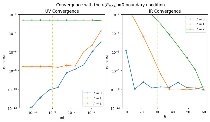
../../_images/50d1824a703e97d12cef10afa937d5cab577cd1783de48e81a82200b6e95dca3.png

On the left, we show the UV convergence for a fixed \(R_\max\), and on the right, we show \(IR\) convergence for a fixed tolerance. We see that the \(n=0\) state is approaching convergence, but that the \(n=1\) and \(n=2\) states have difficulty. The presense of convergence plateaus in one plot indicates that we have reached convergence in the other. On the right plot, we see that choosing an integration tolerance of \(10^{-9}\) allows us to reach this level of precision for all states, but that the \(n=1\) state requires at least \(R_\max > 40\) while the \(n=2\) state requires \(R_\max > 60\).

On the left, we see that a box size of \(R_\max = 30\) allows us to achive high convergence for the \(n=0\) state, but that the \(n=1\) and \(n=2\) states are not converged.

Asymptotic Behaviour#

The IR convergence is best understood by considering the asymptotic behaviour. For large \(r\) we have:

\[\begin{gather*} \lim_{r\rightarrow \infty} \frac{-\hbar^2}{2m} u''(r) \approx E u(r) + \frac{\alpha}{r}u(r). \end{gather*}\]

This introduces two length scales \(a\) and \(r_v\):

\[\begin{gather*} a = \frac{\hbar}{\sqrt{-2m E}}, \qquad r_v = \frac{\alpha}{-E},\qquad \frac{u''(r)}{u(r)} \approx \frac{1}{a^2}\left(1 - \frac{r_v}{r}\right). \end{gather*}\]

The meaning of these is that wavefunction exponential decays with length scale \(a\)

\[\begin{gather*} \lim_{r\rightarrow \infty} u(r) \propto e^{-r/a}. \end{gather*}\]

with a turning point at \(r_v\): \(u''(r_v)\approx 0\).

Notes

Quantitatively, we can include the centrifugal term when solving for \(r_v\):

\[\begin{gather*} a^2r^2\frac{u''(r)}{u(r)} \approx \nu^2 - 1/4 - \frac{2mE}{\hbar^2}r_v - \frac{2m\alpha}{\hbar^2} r \approx (\nu^2 - 1/4)a^2 + r^2 + \frac{\alpha}{E} r,\\ r_v \approx \frac{\alpha}{-E}\frac{1 + \sqrt{1 + (1 - 4\nu^2)\frac{a^2E^2}{\alpha^2}}}{2}. \end{gather*}\]

This will give a better approximation of the turning point for large angular momenta \(l\). We also get a qualitative limit on \(E\) for large \(l\):

\[\begin{gather*} \frac{-\alpha}{a\sqrt{4\nu^2 - 1}} < E < 0 \end{gather*}\]

This can be implemented as the boundary condition:

\[\begin{gather*} au'(R) = -u(R). \end{gather*}\]

def f1(E, **kw):
    """Better objective function encoding long-distance behaviour."""
    a = hbar / np.sqrt(-2*m*E)
    r, u, du = get_r_u_du(E, **kw)
    return a*du[-1] + u[-1]

get_E(Es[1], f=f0, R=20), get_E(Es[1], f=f1, R=20)

(-0.12498711439290973, -0.12499844978860175)

fig, axs = plt.subplots(1, 2, figsize=(10, 5))
ax = axs[0]
for _nE, E in enumerate(Es[:3]):
    Es_ = np.array([get_E(E, f=f1, R=R, tol=_tol) for _tol in tqdm(tols)])
    ax.loglog(tols, abs(Es_/E - 1), '+-', label=f"$n={_nE}$", c=f"C{_nE}")
ax.axvline([tol], c='y', ls=':')
ax.set(xlabel="tol", ylim=(1e-12, 1e-2), ylabel="rel. error", title="UV Convergence")
ax.legend();

ax = axs[1]
for _nE, E in enumerate(Es[:3]):
    Es_ = np.array([get_E(E, f=f1, R=_R, tol=tol) for _R in tqdm(Rs)])
    ax.semilogy(Rs, abs(Es_/E - 1), '+-', label=f"$n={_nE}$", c=f"C{_nE}")
ax.axvline([R], c='y', ls=':')
ax.set(xlabel="R", ylim=(1e-12, 1e-2), ylabel="rel. error", title="IR Convergence")
ax.legend();
plt.suptitle("Convergence with the $u(R_\max) + au'(R)= 0$ boundary condition")
clear_output()
display(fig)
plt.close('all')

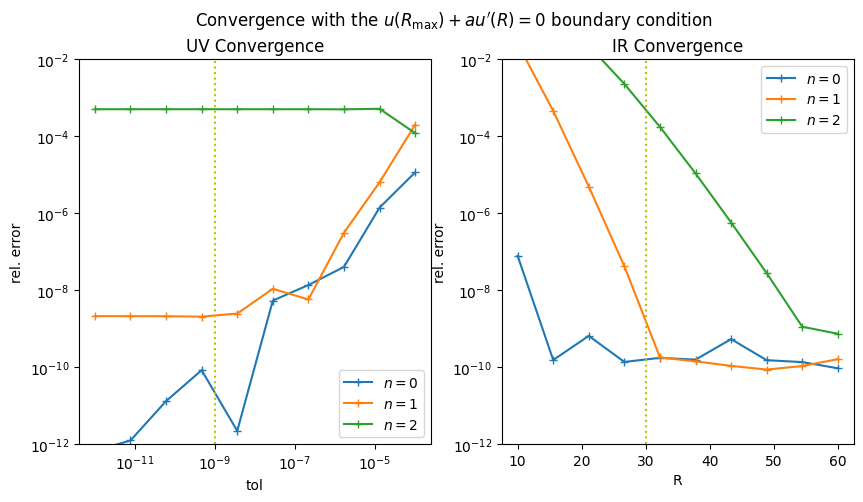
../../_images/6a2ac9cc85a8869f0374ea87a0cbdc368fa18e14bf052b6cc68967b7ea7789a3.png

This gives slightly better behaviour, but it is not dramatic.

A Solution: Integrate Backwards#

The real problem is that, at large \(r\), we have an exponentially diverging solution in addition to the desired exponentially decaying solution. A good strategy is to integrate backwards from a large \(R_\max\) to \(R\): this will quickly dampen any of the exponentially diverging solution, allowing us to match the boundary condition with high accuracy.

What initial conditions should we use? A good strategy is to use the asymptotic form, now including the Coulomb piece to guess. We do a preliminary integration from \(R_\max\) to the turning \(r_v\) to get the scales, then repeat with high accuracy and an initial value so that \(u(r_v) \approx 1\).

How large must \(R_\max\) be? If we want an accuracy of \(\epsilon\), then a good choice is

\[\begin{gather*} \epsilon \approx e^{-{R_\max - r_v}r/a}, \qquad R_\max > r_v - a \ln \epsilon. \end{gather*}\]

def get_r_u_du_backwards(E, u0=None, R=30.0, R_max=None, tol=1e-8, max_step=None, l=0):
    a = np.sqrt(-2*m*E) / hbar
    r_v = max(alpha/(-E), R)   # Could be improved
    if R_max is None:
        R_max = r_v - a * min(-1, np.log(tol))

    if u0 is None:
        # Choose a reasonable initial condition
        if R_max <= r_v:
            u0 = 1
        else:
            u0 = np.sqrt(tol)
            y0 = (u0, -a*u0)        
            res = solve_ivp(partial(compute_du_dr, E=E, l=l), 
                            t_span=(R_max, r_v), 
                            y0=y0, 
                            max_step=(R_max-r_v)/10,
                            atol=tol, rtol=1e-3)
            us_, du_ = res.y
            u0 = us_[0] / us_[-1]
    y0 = (u0, -a * u0)
    R_span = (R_max, R)
    if max_step is None:
        max_step = abs(R_max - R)/10
    res = solve_ivp(partial(compute_du_dr, E=E, l=l), t_span=R_span, y0=y0,
                    max_step=max_step, atol=tol, rtol=tol)
    rs = res.t
    us, dus = res.y
    return rs, us, dus

In principle, one can now integrate both forward an backwards, meeting in the middle.

E = Es[2]
R = 10.0
rs, us, dus = get_r_u_du(E, R=R)
rs_, us_, dus_ = get_r_u_du_backwards(E, R=R)
plt.plot(rs, us)
plt.plot(rs_, us_*us[-1]/us_[-1])

[<matplotlib.lines.Line2D at 0x7f525813e0d0>]

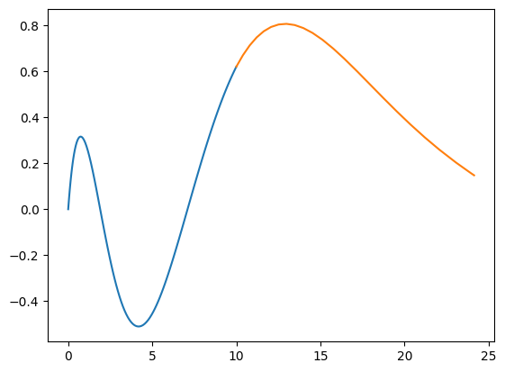
../../_images/e42574a5b8b5c0726cfbd7799415228d03f2e13157c7099162f4aa71236bbe7e.png

We now show that it is sufficient to run the backwards iteration. As running to \(r=0\) is slightly problematic, we choose a small \(r_0\) and then do a polynomial extrapolation of the last few points to extrapolate to \(r=0\), requiring that \(\lim_{r\rightarrow 0} u(r) = 0\).

Notes:

Using the simple condition \(r_0 u'(r_0) - u(r_0) = 0\) corresponds to a linear extrapolation of the last two points, but does not give high precision, even if \(r_0\) is carefully chosen. (This is the usual issue of balancing truncation and roundoff errors).
The parameters in the default version have been tweaked a bit by hand exploring up to the \(n=7\) hydrodgen solution. This could be done a bit better.

def f_(E, ar0=1e-2, aR_max=None, N=10, order=6, **kw):
    a = hbar/np.sqrt(-2*m*E)
    if aR_max is None:
        R_max = None
    else:
        R_max = aR_max * a
    r0 = ar0 * a
    rs_, us_, dus_ = get_r_u_du_backwards(E, R=r0, R_max=R_max, **kw)
    return np.polyval(np.polyfit(rs_[-N:], us_[-N:], deg=order), 0)/abs(us_).max()
    return (r0*dus_[-1] - us_[-1])/np.sqrt((r0*dus_[-1])**2 + (us_[-1])**2)

print(np.abs(list(map(partial(f_, aR_max=20), Es))).max())
print(np.abs(list(map(partial(f_, aR_max=40), Es))).max())
print(np.abs(list(map(partial(f_, aR_max=50), Es))).max())
print(np.abs(list(map(partial(f_, aR_max=60), Es))).max())
print(np.abs(list(map(partial(f_, aR_max=100), Es))).max())

print(np.abs(list(map(partial(f_, aR_max=20), Es))).max())
print(np.abs(list(map(partial(f_, aR_max=40), Es))).max())
print(np.abs(list(map(partial(f_, aR_max=50), Es))).max())
print(np.abs(list(map(partial(f_, aR_max=60), Es))).max())
print(np.abs(list(map(partial(f_, aR_max=100), Es))).max())

0.09766075090362927

0.008539092320768528

2.5366768527963025e-06

1.2099897998722325e-08

0.022856750399549985

ns_ = np.linspace(0.8, 20, 200)
Es_ = -m*alpha**2/2/hbar**2/ ns_**2
fs_ = np.array(list(map(partial(f_), tqdm(Es_))))
fig, ax = plt.subplots(figsize=(10, 5))
ax.plot(ns_, fs_)
ax.grid(True)
ax.set(xlabel="$n$", ylabel="boundary condition", xticks=np.arange(20));

  0%|          | 0/200 [00:00<?, ?it/s]

  6%|▌         | 11/200 [00:00<00:01, 105.02it/s]

 11%|█         | 22/200 [00:00<00:01, 104.98it/s]

 16%|█▋        | 33/200 [00:00<00:01, 100.99it/s]

 22%|██▏       | 44/200 [00:00<00:01, 92.52it/s]

 27%|██▋       | 54/200 [00:00<00:01, 82.11it/s]

 32%|███▏      | 63/200 [00:00<00:01, 74.89it/s]

 36%|███▌      | 71/200 [00:00<00:01, 69.18it/s]

 40%|███▉      | 79/200 [00:01<00:01, 63.04it/s]

 43%|████▎     | 86/200 [00:01<00:01, 58.29it/s]

 46%|████▌     | 92/200 [00:01<00:01, 54.34it/s]

 49%|████▉     | 98/200 [00:01<00:02, 50.79it/s]

 52%|█████▏    | 104/200 [00:01<00:02, 47.69it/s]

 55%|█████▍    | 109/200 [00:01<00:02, 45.31it/s]

 57%|█████▋    | 114/200 [00:01<00:02, 42.89it/s]

 60%|█████▉    | 119/200 [00:02<00:01, 41.16it/s]

 62%|██████▏   | 124/200 [00:02<00:01, 39.35it/s]

 64%|██████▍   | 128/200 [00:02<00:01, 37.80it/s]

 66%|██████▌   | 132/200 [00:02<00:01, 36.66it/s]

 68%|██████▊   | 136/200 [00:02<00:01, 35.23it/s]

 70%|███████   | 140/200 [00:02<00:01, 33.79it/s]

 72%|███████▏  | 144/200 [00:02<00:01, 32.56it/s]

 74%|███████▍  | 148/200 [00:02<00:01, 31.82it/s]

 76%|███████▌  | 152/200 [00:03<00:01, 30.97it/s]

 78%|███████▊  | 156/200 [00:03<00:01, 30.39it/s]

 80%|████████  | 160/200 [00:03<00:01, 29.83it/s]

 82%|████████▏ | 163/200 [00:03<00:01, 29.22it/s]

 83%|████████▎ | 166/200 [00:03<00:01, 28.53it/s]

 84%|████████▍ | 169/200 [00:03<00:01, 28.00it/s]

 86%|████████▌ | 172/200 [00:03<00:01, 27.45it/s]

 88%|████████▊ | 175/200 [00:03<00:00, 26.92it/s]

 89%|████████▉ | 178/200 [00:04<00:00, 26.40it/s]

 90%|█████████ | 181/200 [00:04<00:00, 25.95it/s]

 92%|█████████▏| 184/200 [00:04<00:00, 25.37it/s]

 94%|█████████▎| 187/200 [00:04<00:00, 24.97it/s]

 95%|█████████▌| 190/200 [00:04<00:00, 24.61it/s]

 96%|█████████▋| 193/200 [00:04<00:00, 23.91it/s]

 98%|█████████▊| 196/200 [00:04<00:00, 23.72it/s]

100%|█████████▉| 199/200 [00:04<00:00, 23.54it/s]

100%|██████████| 200/200 [00:04<00:00, 40.44it/s]

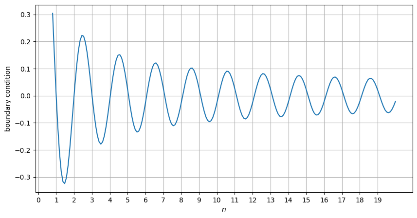
../../_images/a380f77d9c0d6b8b55167c31f87743c26d60dd621b45d0a2196055fd42d94674.png

From the previous plot, we see that the normalized boundary condition is very regular, lending itself to nice root-finding.

Es = -m*alpha**2/2/hbar**2/ np.arange(1, 10)**2
#get_E(Es[-1], f=f_, tol=1e-9)/Es[-1] - 1

# Broken if tol too large... check
get_E(Es[-1], f=f_, tol=1e-8)/Es[-1] - 1

-0.019447742012686953

E = Es[-1]
a = np.sqrt(-2*m*E)/hbar
r, u, du = get_r_u_du_backwards(E=E, R=0.1/a, R_max=60/a, u0=1e-12, tol=1e-10, max_step=)
plt.plot(r, u, '+')
axis = plt.axis()
plt.plot(r, 1e10*np.exp(-a*r))
plt.axis(axis)

from scipy.integrate import solve_bvp
def compute_du_dr_E(r, u_, E_):
    E, = E_
    du, ddu = compute_du_dr(r, u_, E=E)
    return du, ddu

def bc(u0_, uR_, E_):
    E, = E_
    a = np.sqrt(-2*m*E)/hbar
    u0, du0 = u0_
    uR, duR = uR_
    return (u0, du0 - 1, a*duR + uR)

E = Es[0]
a = np.sqrt(-2*m*E)/hbar
r0 = 1e-3/a
R_max = 60.0/a
r = np.linspace(r0, R_max)
u = r*np.exp(-a*r)
du = (1-a*r)*np.exp(-a*r)
sol = solve_bvp(compute_du_dr_E, bc, x=r, y=(u, du), p=[E], tol=1e-12, bc_tol=1e-12)
r = sol.x
u, du = sol.y
E_ = sol.p[0]
plt.plot(r, u), E/E_
#bc((u[0], du[0]), (u[-1], du[-1]), [E])

from tqdm import tqdm

Es = -m*alpha**2/2/hbar**2/ np.arange(1, 5)**2

tols = 10**(np.linspace(-4, -12, 10))
aRs = np.linspace(10.0, 60.0, 10)
aR = 30.0
tol = 1e-6

fig, axs = plt.subplots(1, 2, figsize=(10, 5))
ax = axs[0]
for _nE in reversed([0, 1, 2, len(Es)-1]):
    E = Es[_nE]
    Es_ = np.array([get_E(E, f=f_, aR_max=aR, tol=_tol) for _tol in tqdm(reversed(tols))])
    axs[0].loglog(tols, abs(Es_/E - 1), '+-', label=f"$n={_nE}$", c=f"C{_nE}")

    Es_ = np.array([get_E(E, f=f_, aR_max=_aR, tol=tol) for _aR in tqdm(reversed(aRs))])
    axs[1].semilogy(aRs, abs(Es_/E - 1), '+-', label=f"$n={_nE}$", c=f"C{_nE}")

axs[0].axvline([tol], c='y', ls=':')
axs[0].set(xlabel="tol", ylim=(1e-12, 1e-2), ylabel="rel. error", title="UV Convergence")
axs[0].legend();

axs[1].axvline([R], c='y', ls=':')
axs[1].set(xlabel="R", ylim=(1e-12, 1e-2), ylabel="rel. error", title="IR Convergence")
axs[1].legend();

plt.suptitle("Convergence with the $u(R_\max) + au'(R)= 0$ boundary condition")
clear_output()
display(fig)
plt.close('all')

How to Solve the Schrödinger Equation (Old)#

We will consider here only spherically symmetric problems for simplicity. We start with some numerical code to solve the radial Schrödinger equation. We do this in two ways: one with finite differences (easy to code, but not very accurate), and once with a Bessel-function discrete variable representation (DVR) basis as described in [Littlejohn and Cargo, 2002]. The latter is a very accurate spectral method, (exponentially accurate for analytic potentials) but might seem like a bit of a black box until you study DVR bases a bit more.

Radial Equation#

With the usual spherical coordinates \(\phi\) and \(\theta\), and angular momentum quantum numbers \(l\) and \(m\), we have

\(d\)	\(\Omega\)	\(\lambda\)
\(2\)	\(\phi\)	\(\abs{m}\)
\(3\)	\((\phi, \theta)\)	\(l\)

for \(d=2\) dimensions (i.e. cylindrical coordinates, but no \(z\) dependence) and \(d=3\) dimensions respectively. The total orbital angular momentum operator is related to the Laplace-Beltrami operator by

\[\begin{gather*} \op{L}^2 = \hbar^2\op{\Delta}_{S^{d-1}} \end{gather*}\]

which has eigenvalues \(\hbar^2 m^2\) in \(d=2\) (i.e. \(\op{L}^2 \equiv \op{L}_z^2\) and \(\hbar^2 l (l - 1)\) in \(d=3\).

Our aim is to satisfy the Schrödinger equation for central potentials in \(d\)-dimensions, which we can do in the usual way by expressing the wavefunction \(\Psi(r, \Omega) = \psi(r)Y_{\lambda}(\Omega)\) in terms of the radial wavefunction \(u(r)\) and the appropriate generalized spherical harmonics \(Y_{\lambda}(\Omega)\):

\[\begin{gather*} \left(\frac{-\hbar^2\nabla^2}{2m} + V(r) - E\right)\Psi(r, \Omega) = 0, \\ \left[ \frac{\hbar^2}{2m} \underbrace{ \left(-\diff[2]{}{r} + \frac{\nu^2 - 1/4}{r^2}\right) }_{\op{K}} + V(r)\right]u(r) = E u(r),\\ u(r) = r^{(d-1)/2}\psi(r), \qquad \nu = \lambda + \frac{d}{2} - 1. \end{gather*}\]

Details

Here \(\Omega\) is the generalized solid angle. Rotational invariance implies that angular momentum is a good quantum number, so all eigenstates can be factored \(\Psi(r, \Omega) = \psi(r)Y_{\lambda}(\Omega)\) where \(Y_{\lambda}(\Omega)\) is the generalized spherical harmonic on the (\(d-1\))-dimensional sphere and \(\lambda \in \{0, 1, \dots\}\) is the generalized angular momentum:

\[\begin{gather*} \nabla^2 = \frac{1}{r^{d-1}}\diff{}{r}\left(r^{d-1} \diff{}{r}\right) + \frac{1}{r^2}\Delta_{S^{d-1}}, \\ \Delta_{S^{d-1}}Y_{\lambda}(\Omega) = \lambda (\lambda + d - 2)Y_{\lambda}(\Omega), \end{gather*}\]

where \(\Delta_{S^{d-1}}\) is the Laplace-Beltrami operator. Introducing the radial wavefunction \(u(r)\), this becomes quadratic:

\[\begin{gather*} u(r) = r^{(d-1)/2}\psi(r), \qquad \nu = \lambda + \frac{d}{2} - 1,\\ r^{(d-1)/2}\nabla^2 \psi(r) = \left(\diff[2]{}{r} - \frac{\nu^2 - 1/4}{r^2}\right)u(r). \end{gather*}\]

This follows after a little algebra from

\[\begin{gather*} \frac{1}{r^{d-1}}\diff{}{r}\left(r^{d-1} \diff{}{r}\right)r^{(1-d)/2}u(r)\\ = r^{(1-d)/2} \left( \diff[2]{}{r} - \frac{(d-3)(d-1)}{4} \right)u(r). \end{gather*}\]

This can be solved quite simply – but not very accurately – with finite differences. Highly accurate solutions can be obtained by shooting, but this can be inefficient. I highly recommend that you stop and implement your own solution to this problem for various functions \(V(r)\) and parameters \(\nu\). As a check, you should be able to find the eigenstates for hydrogenic atoms with \(V(r) \propto 1/r\).

from phys_581 import seq
from importlib import reload
reload(seq)

class SEQ(seq.CoulombSEQ):
    """Classic Coulomb potential."""
    hbar = m = 1
    alpha = 1.0

    def V(self, r):
        return -self.alpha / r
    
    def get_E0(self, ns, l=0):
        """"Return the exact energies for hydrogen."""
        E_Ry = -self.m * self.alpha**2 / 2 / self.hbar**2
        return E_Ry / (ns + l + 1)**2

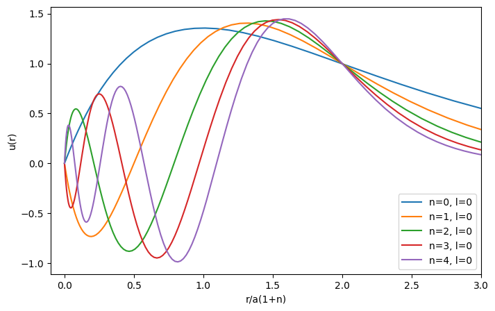
    def plot(self, N=None, Es=None,l=0, fig=None):
        """Plot N wavefunctions"""
        if Es is None:
            Es = self.get_E0(ns=np.arange(N), l=l)
    
        if fig is None:
            fig, ax = plt.subplots(figsize=(8,5))
        else:
            ax = fig.gca()
        
        for n, E in enumerate(Es):
            r, u, du = self.get_r_u_du_backwards(E=E)
            ax.plot(r/(1+n)/self.get_a(E=E), u, label=f"n={n}, l={l}")
        ax.set(xlabel="r/a(1+n)", ylabel="u(r)", xlim=(-0.1, 3))
        ax.legend()
        return fig

s = SEQ()
l = 0
s.plot(5, l=l);

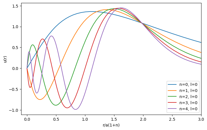
../../_images/6cb3615a250c18d8efc93f3c6ba444fce23c187a798eb33eaedcce2c2fce6ddd.png

class SEQ1(SEQ):
    """Truncated Coulomb potential."""
    r0 = 0.5
    V0 = None
    
    def V(self, r):
        V0 = self.V0
        if V0 is None:
            V0 = super().V(self.r0)
        return np.where(r<self.r0, V0, super().V(r))
    
    def plot(self, N, l=0, **kw):
        E0s = super().get_E0(ns=np.arange(N), l=l)
        Es = [self.compute_E(_E, l=l) for _E in E0s]
        super().plot(Es=Es, **kw)
    
s1 = SEQ1()
s1.plot(5, l=l);

../../_images/534ce3d14bd26e3098a1b624e6536218ffe6b2e06a9fb3c8deac6cda6002fcd0.png

k = 2*np.pi * np.fft.fftfreq(N, dx)
K = (hbar*k)**2/2/m
A = np.fft.ifft(K*np.fft.fft(np.eye(N), axis=1), axis=1)
V = np.diag(Vx)
C = None

E, psi = sp.linalg.eig(A+V, C)
inds = np.argsort(abs(E))
E, psi = E[inds], psi[:, inds]
E[:10].real

---------------------------------------------------------------------------
NameError                                 Traceback (most recent call last)
Cell In[16], line 1
----> 1 k = 2*np.pi * np.fft.fftfreq(N, dx)
      2 K = (hbar*k)**2/2/m
      3 A = np.fft.ifft(K*np.fft.fft(np.eye(N), axis=1), axis=1)

NameError: name 'N' is not defined